Surface Mesh
Introduction
Now that we have a geometry, we can start meshing it. We are using Pointwise to generate the surface mesh. This is not a full blown tutorial, more a walk through. If you want to learn more about it, their Youtube channel is highly recommended. You do not have to use Pointwise to generate an overset mesh. ICEM or an other meshing software would work as well.
Files
Navigate to the directory overset/mesh in your tutorial folder. Either use the previously generated .igs file or copy it from the tutorial folder.
cp ../../../tutorial/overset/geo/onera_m6.igs .
It is possible to script Pointwise. In order to use it, we have to download the script first. You can either download it here or copy it from the tutorial folder.
cp ../../../tutorial/overset/mesh/Semicircle.glf .
Meshing strategy
Before we start meshing, we have to know how many meshes we create and where they overlap. For this tutorial,
3 different meshes are proposed: near_wing, near_tip and far. The following picture should give an overview:
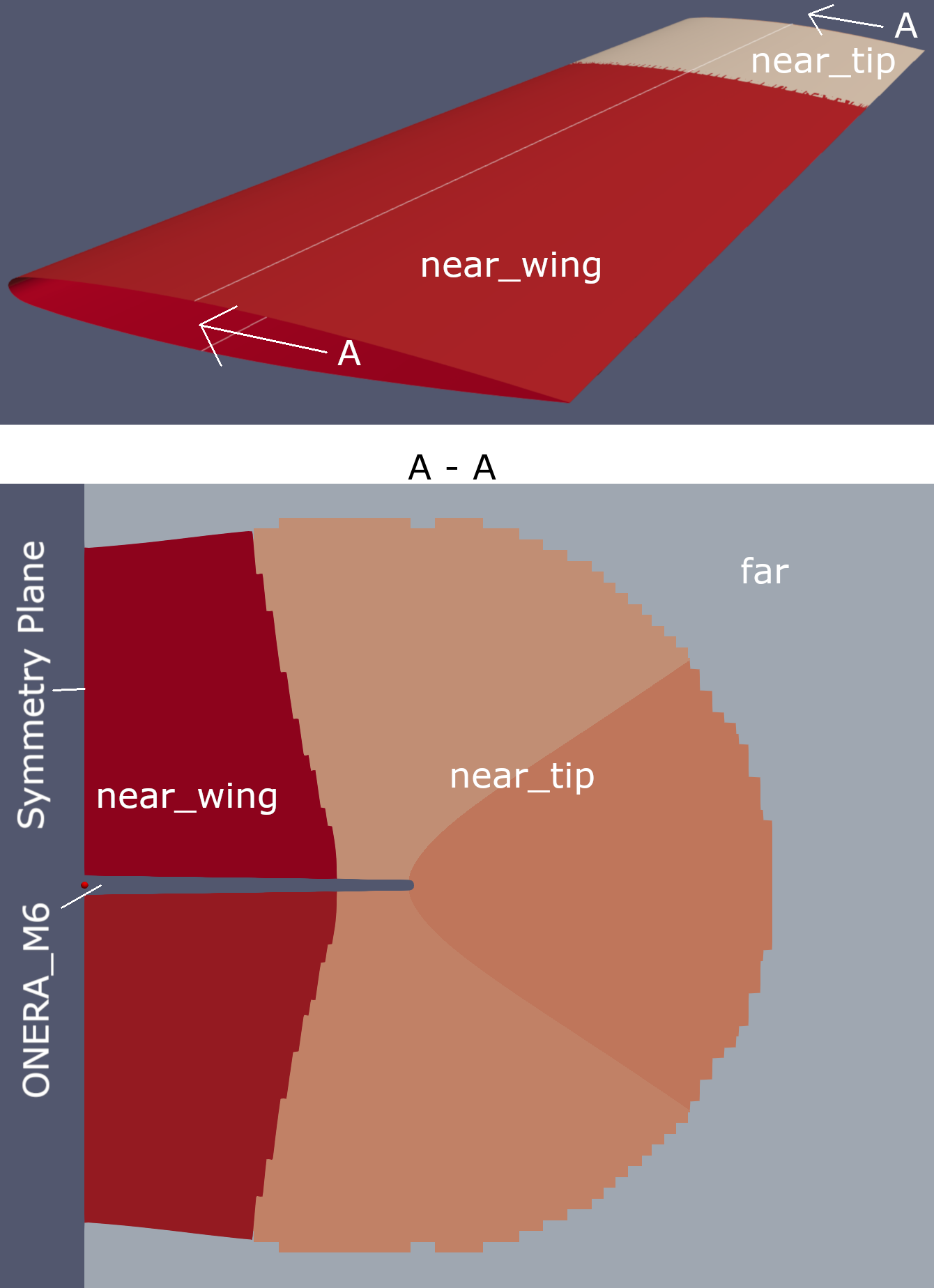
The three overset meshes.
Now we should estimate the cell count of the mesh. For the purpose of a grid convergence study (GCS) and debugging it makes sense to have differently refined meshes. To limit the amount of work, we will create the finest mesh and coarsen it multiple times.
Usually, the finest mesh is called L0 (level 0) and should have approx 60M cells for this geometry. If every 2 cells
are combined in each direction, we get a coarser mesh called L1. This usually goes to L2 for production and L3 for
debugging purposes. Additionally, there could be an intermediate level starting at L0.5. It requires a different
surface mesh that is sqrt(2) coarser than L0. In this tutorial, we will start at L1 (~8M cells) and end at L3
(~0.125M cells).
Mesh Generation
Pointwise overview
If you start Pointwise, it should look something like in the next picture.
Object, Layer and Default control
Solver information
Selection control
View control
Fast meshing controls
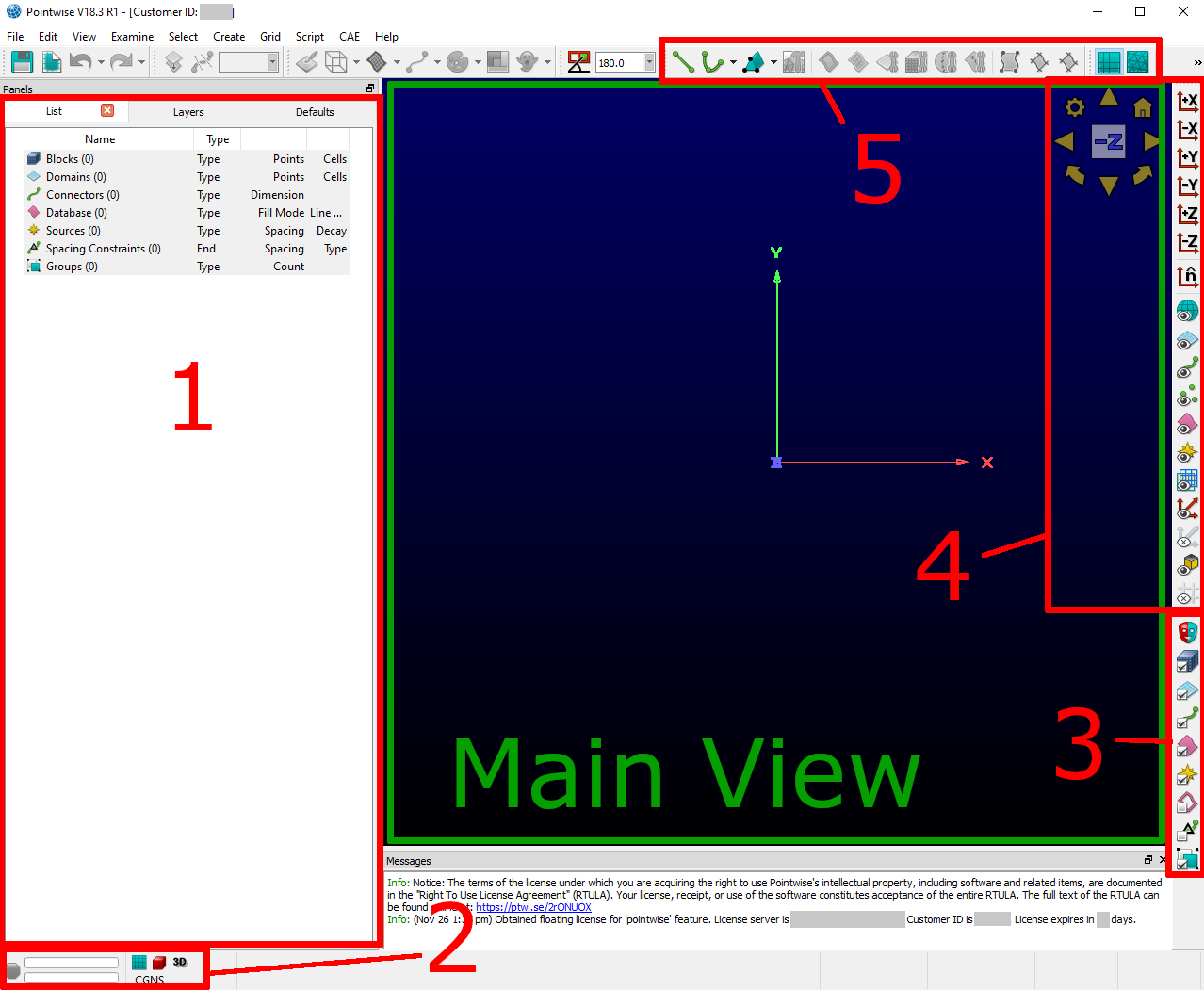
Pointwise Overview.
You can control the main view with the following key- and mouse combinations:
- zoom
Rotate your
mouse wheel. The zoom centers around yourmouse pointer.- rotate
Press
ctrland yourright mouse buttonwhile moving your mouse.- move
Press
shiftand yourright mouse buttonwhile moving your mouse.
Setup Pointwise
Before we actually begin meshing, we have to set some standard values and import our geometry. At first, we set some tolerances for Pointwise
Click on
File->PropertiesSet
Model Sizeto1. (It is enough, if the order of magnitude is similar)Set
Nodeto1e-6. The value ofConnectorshould automatically jump to1e-6as wellOK
Now we have to choose the proper solver. In my case it is CGNS with adf support. If you have compiled the
MACH-Framework with hdf5 support, you can skip the last step.
Click
CAE->Select SolverMake Sure
CGNSis selected.Click
OK.Click
CAE->Set Dimension->2D(That’s how surface meshes are called here)Click
CAE->Set Solver Attributes(If you havehdf5support, you can stop here)Select
adfforCGNS File TypeClick
Close
Now we can import the .iges file we created in the previous tutorial.
Click
File->Import->DatabaseSelect your
.igesFile ->openMake sure nothing but
UnitsandFrom Fileis selectedClick
OKYou will receive a warning that some entities could not be converted. Just ignore it and click
YES
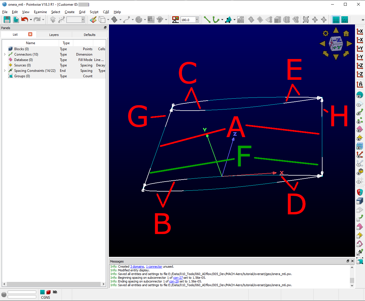
After those steps, the window should look like this (you should probably save at this point):
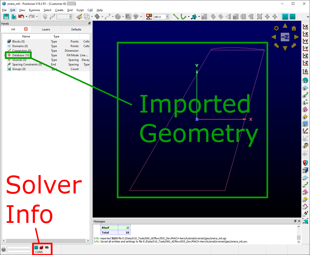
Pointwise after setup.
Few important Pointwise labels:
- Block
This is a 3 dimensional Mesh
- Domain
This is a 2 dimensional Mesh
- Connector
A line constraining the extend of a
BlockorDomain- Database
An imported geometry
- Spacing Constraint
This controls how the
nodeslay on aConnector. Further down the line, theConnectorcontrols how thenodeslay in aDomainorBlock
Prepare the Database
To make our live a bit easier in the coming mesh work, we first prepare the database a bit (take a look at the next picture to help guide you).
Select the whole
database. Just draw a rectangle around it while yourleft mouse buttonis pressedClick
Wireframe->ShadedClick on
LayersDouble click on
Descriptionand enterGeo
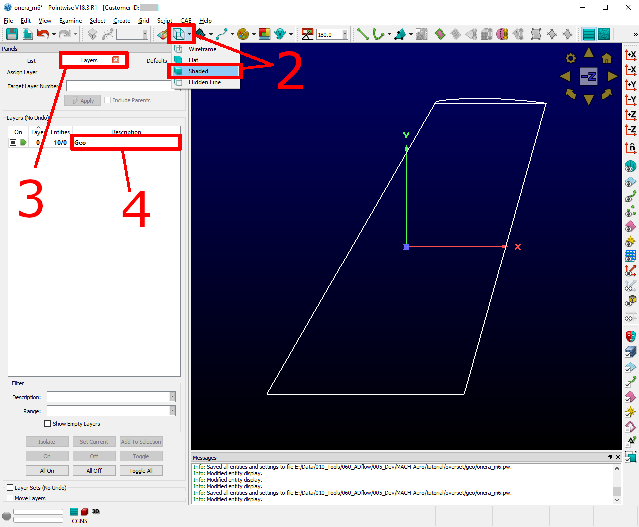
Prepare the database #1.
Because we have two overlapping meshes (near_wing and near_tip), we have to cut the database at an appropriate place.
This will indicate where the near_tip mesh will start. The near_wing mesh will go right to the tip of the wing. But
because ADflow uses an Implicit Hole Cutting Scheme we only have to make sure, that the near_tip mesh is slightly smaller
than the near_wing mesh. This will ensure, that the overlapping region is approximately where we cut the database. In this
way we are certain, the solver does not have to interpolate in a critical region (like the wing tip).
Click on
Create->PlanesChoose
Constant X, Y or ZSelect
Yand enter a value of0.9Click
OK(Your view should now look like detailAin the following picture)Select only the
upper,lowerandtrailing edgesurface by drawing a rectangle with yourleft mouse buttonClick
Edit->Trim by SurfacesSelect your freshly created plane (detail
A)Make sure
ToleranceandAdvancedis unselectedClick
Imprint(Your geometry should now have a different color towards the tip)Click
OK
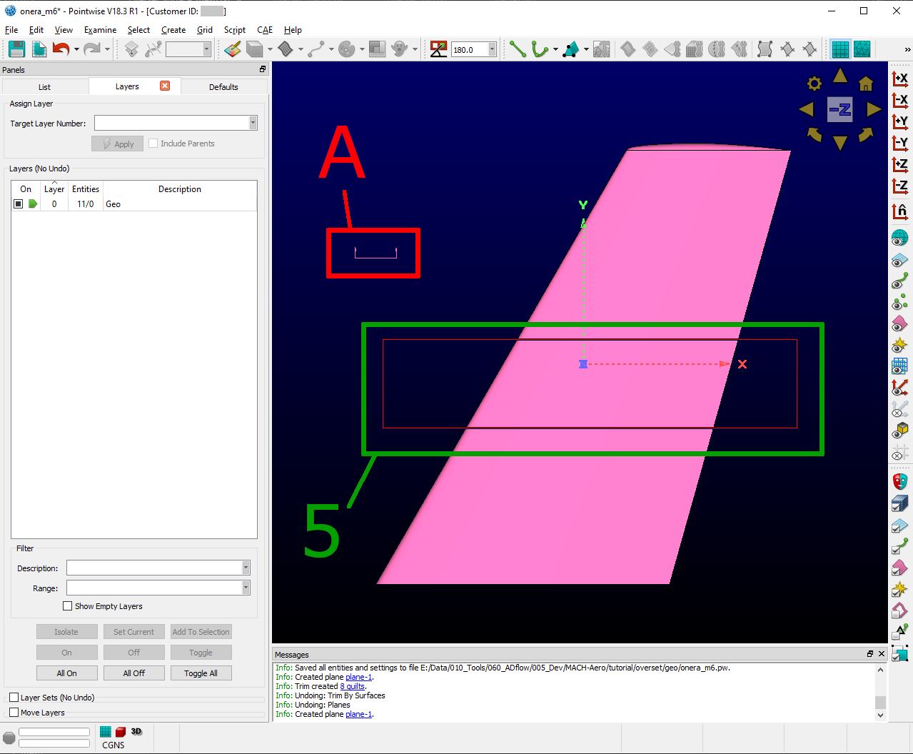
Cut the database.
Now we are doing some cleaning up and delete some unneeded surfaces.
Rotate your view with pressing
ctrland yourright mouse buttonwhile moving your mouse until you have a good view on the root surfaces.Select the first
root surfacePress
ctrlwhile selecting the secondroot surfacePress
delon your keyboard to delete them
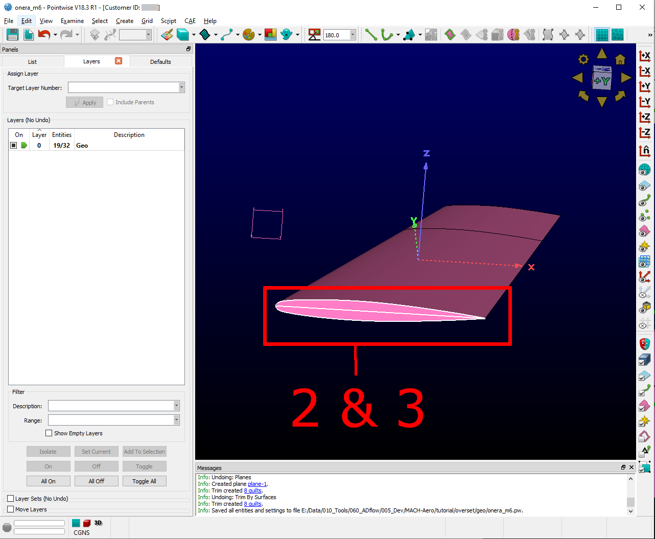
Delete the root surfaces.
Create the near_wing surface mesh
We create the mesh near_wing in a new layer to keep everything orderly.
Click
LayersSelect
Show Empty LayersClick with your
right mouse buttonon layer10->Set CurrentDouble click with your
left mouse buttonon theDescriptionof layer10and enternear_wingUnselect
Show Empty Layers
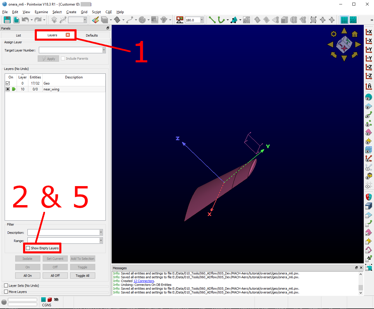
Create a new layer for near_wing.
Because we want to coarsen our mesh multiple times, it is important to think about how many nodes we should have on a connector (Apart from that, it is always good to be multi-grid-friendly). To calculate the number of nodes (\(N\)) per connector, we use this formula:
Where \(n\) is the number of refinements + 1 and \(m\) is an integer. For our chord-wise direction, we will
use ‘’145’’ Nodes. To save some work, we will set it as default.
Click
DefaultsMake sure
Connectoris checkedSelect
Dimensionand enter145Select the
upperandlowersurface of the wingClick
Connectors on Database EntitiesClick on
Layersand uncheck theGeolayerSelect the
two connectorsin the middle of the wing (Detail A) and delete them. They showed up because we split the databaseSelect the
6 spanwise connectors(Detail B)Click
Edit->Join
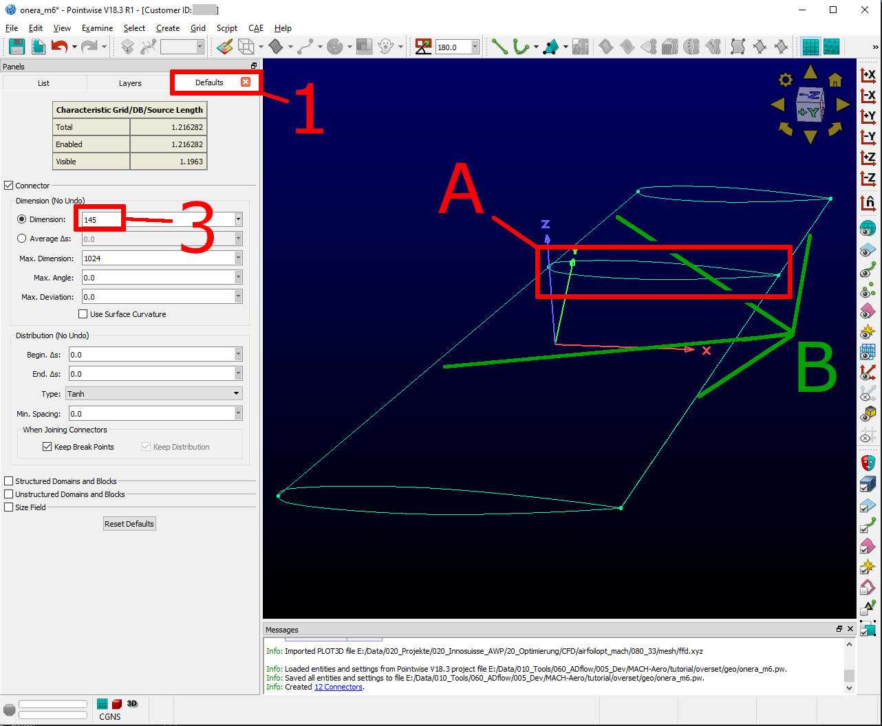
Create the connectors for the near_wing mesh.
When creating the connectors, we left out the TE. We did this because there were 2 surfaces from OpenVSP. It is less work for us, if we manually create two connectors.
Click
DefaultsSelect
Dimensionand enter17Click
2 Point CurvesClose the
root trailing edge(make sure your pointer becomes a cross-hair before you click. This way you are sure the new connector lies on the closest point)Close the
tip trailing edgePress
OK
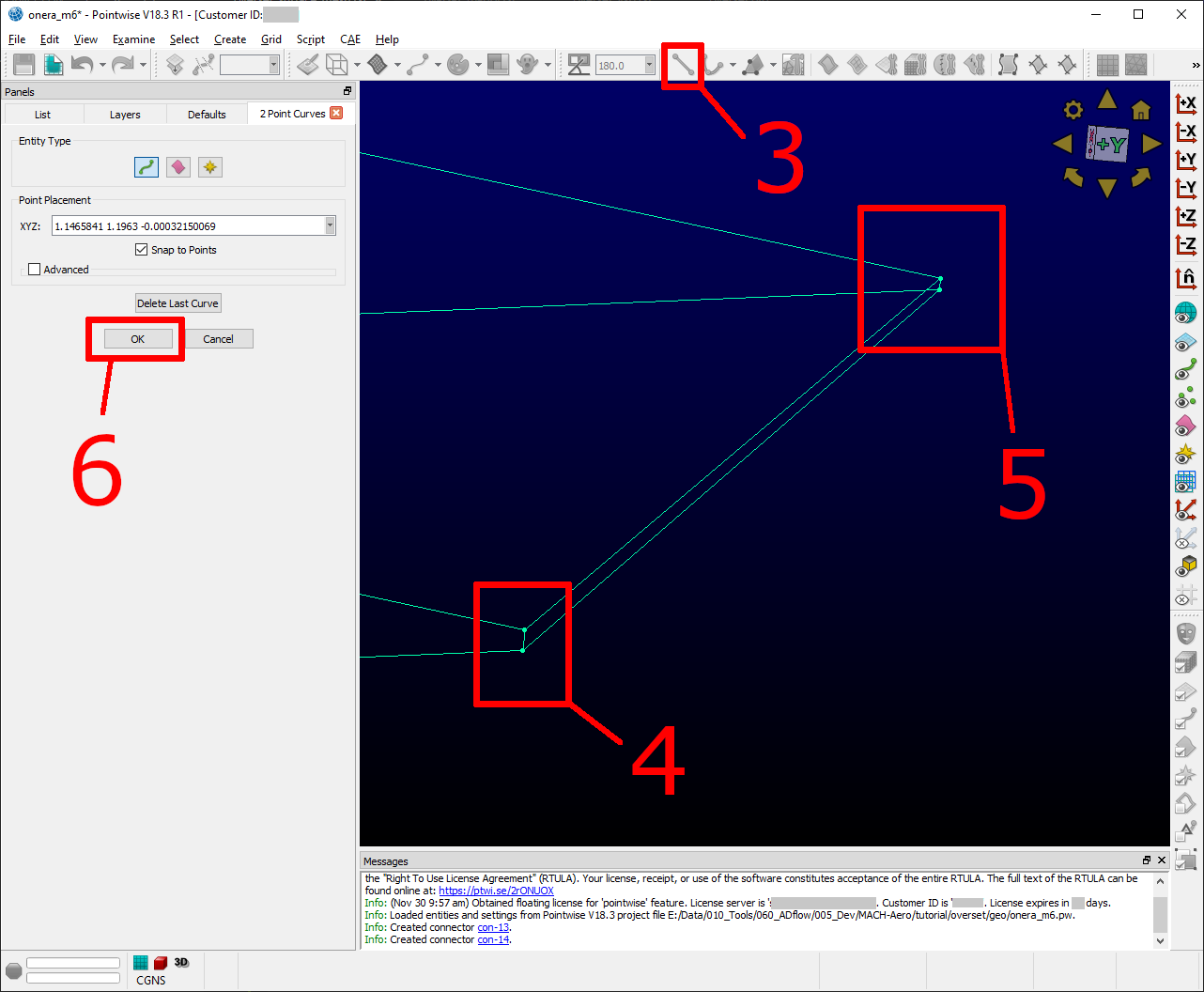
Close the trailing edge.
Now we initialize the surface mesh.
Select
everythingClick
Assemble DomainsSelect
everythingClick on the
small arrow pointing downnext toWireframeClick on
Hidden Line
Initialize the near_wing mesh.
Now we size the LE (Leading Edge) and TE (Trailing Edge) connectors.
Click on
All Masks On/OffClick on
`ConnectorsSelect the
LEandTEConnectorsby drawing a rectangle like it is shownClick on the input field next to
Dimension, enter73and hitenter
Dimension the LE & TE connectors.
The surface mesh is now almost complete. We only have to distribute the nodes on it properly by changing the spacing.
Usually all Points are distributed according to Tanh. But because we split up the database in the previous steps,
we have to remove so called break point at that location.
Note
Break Points give you even more control to distribute your nodes on a connector.
Select the
LEandTEconnectors again.Click on
Grid->DistributeClick on
Break PointsClick on
Delete all Break PointsClick on
OK
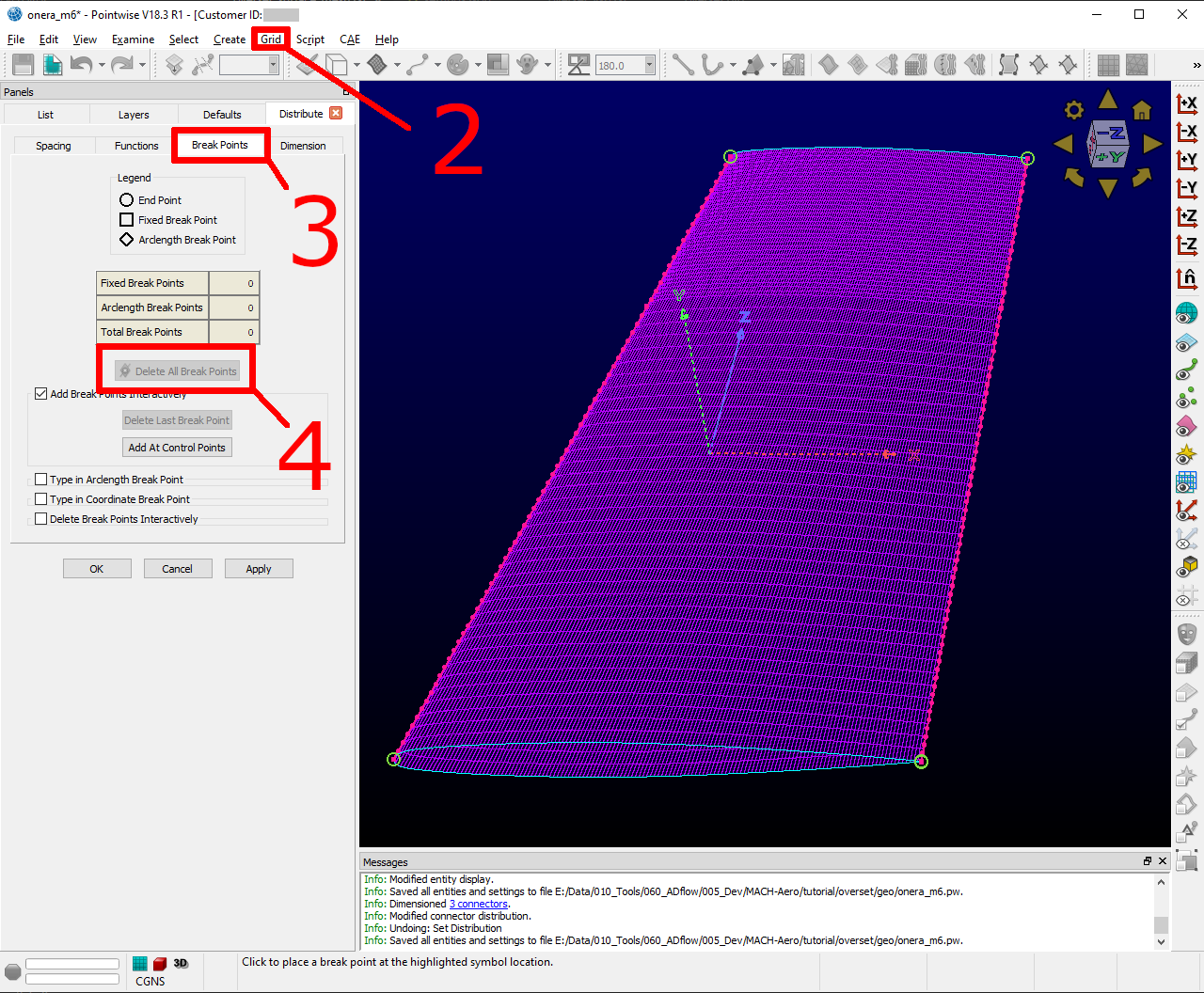
Delete unneeded Break Points.
Click on
All Masks On/OffClick on
Spacing ConstraintsSelect the 2 spacing constraints at the
LEof theroot(A)Click the field next to
Spacingand enter0.0003. Then hitenterSelect the 2 spacing constraints at the
TE root(B)Apply
7.15e-5for spacingSelect the 2 spacing constraints at the
LE tip(C)Apply
0.00016for spacingSelect the 2 spacing constraints at the
TE tip(D)Apply
4e-5for spacingSelect the 3 spacing constraints at the
tip(E)Apply
0.0025for spacingSelect the 3 spacing constraints at the
root(F)Apply
0.04as spacing
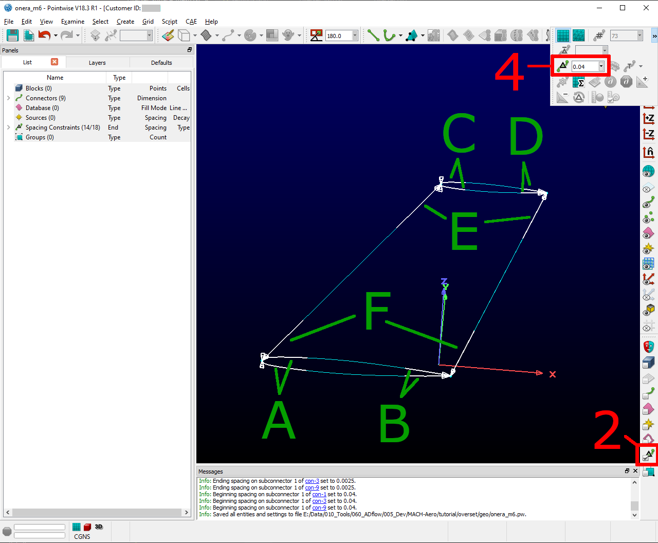
Apply the proper spacing.
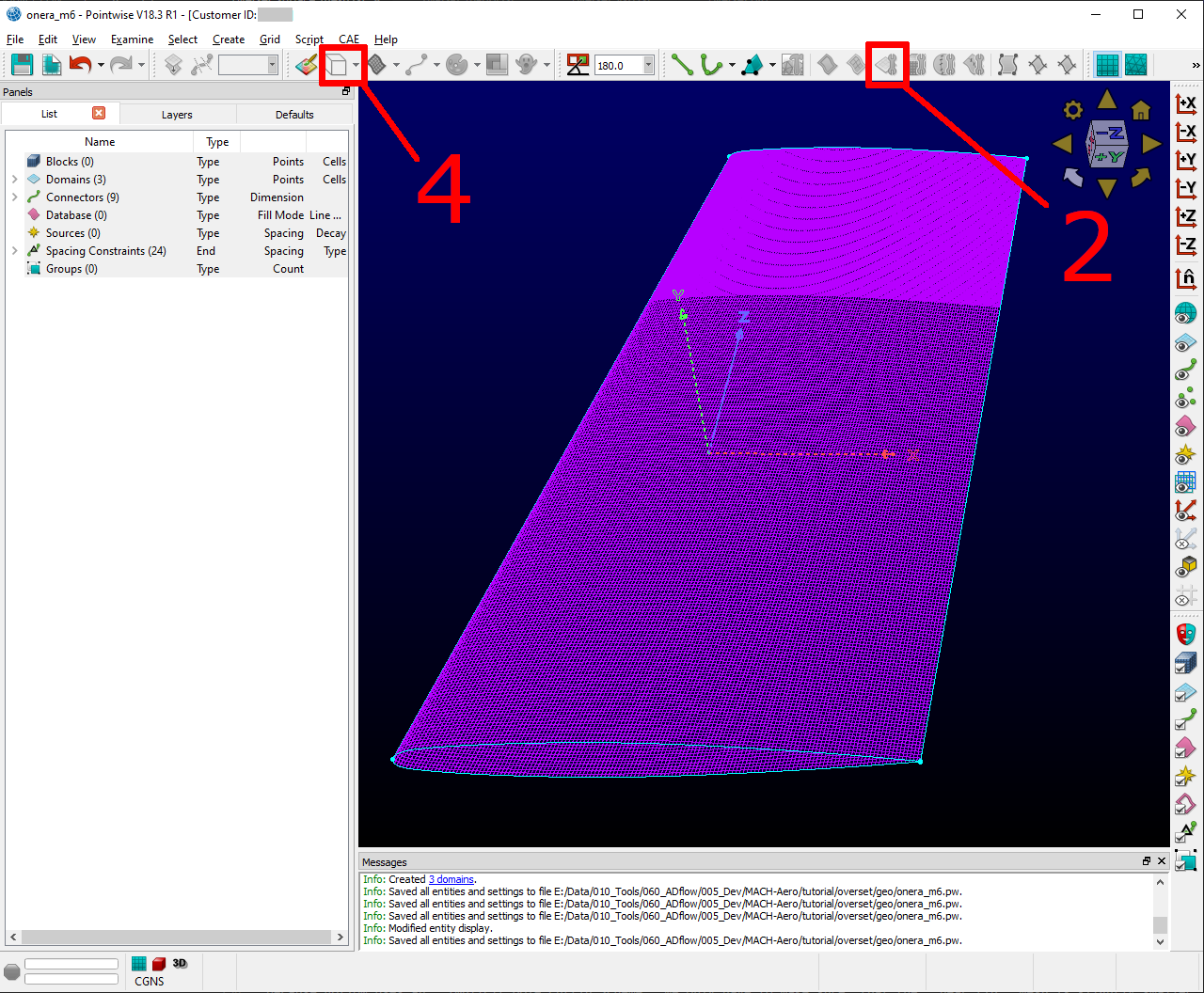
The mesh near_wing is now complete. We will export it later.
Create the near_tip surface mesh
Now we will create the near_tip mesh. Let’s start with creating a new layer and hide everything unnecessary.
Click on
LayersCheck
Show Empty LayersRight click on Layer
20->Set CurrentDouble click the
DescriptionField and enternear_tipUncheck
Show Empty LayersCheck Layer
0to make the database visibleHide the mesh
near_wingby un-checking layer10
Now we will create the connectors.
Click on
Defaults-> enter201forDimensionSelect everything from the tip to the cut we made earlier
Click
Connectors on Database EntitiesClick on
Layers-> uncheck layer0. Now, you should only see the connectors we created
Let’s clean up the generated connectors at the tip TE.
Zoom into the
tip TESelect the
5shownconnectors(A)Delete them
Select and delete the remaining
pole(the point with a circle around) (B)Select the
2connectorsthat define the outer tip (C)Click
Edit->JoinSelect the
newly joinedconnector (C)Enter
65ForDimensionand hitenterClick on
Defaultsand enter65forDimensionClick on
2 Point CurvesClose the
TEagain (D)
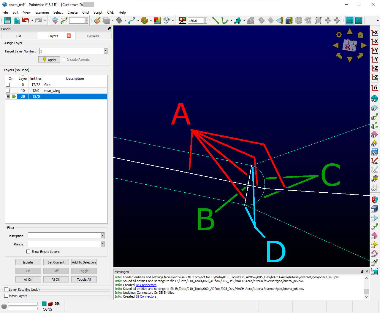
Clean up the tip TE.
Next we clean up the root TE.
Select the
2connectorsthat define the TE (A)Delete them
Click on
2 Point CurvesClose the Tip again (B)
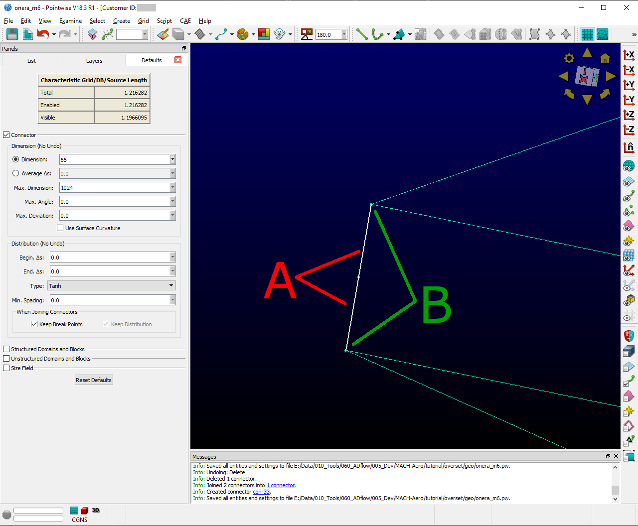
Clean up the root TE.
The last thing to clean up is the tip LE.
Select the
3shownconnectors(A)Click on the
arrow pointing downnext toshowClick
HideSelect and delete the remaining
pole(B)Click on
View->Show HiddenSelect the
3connectors(A)Click on the
arrow pointing downnext toHideClick on
Show
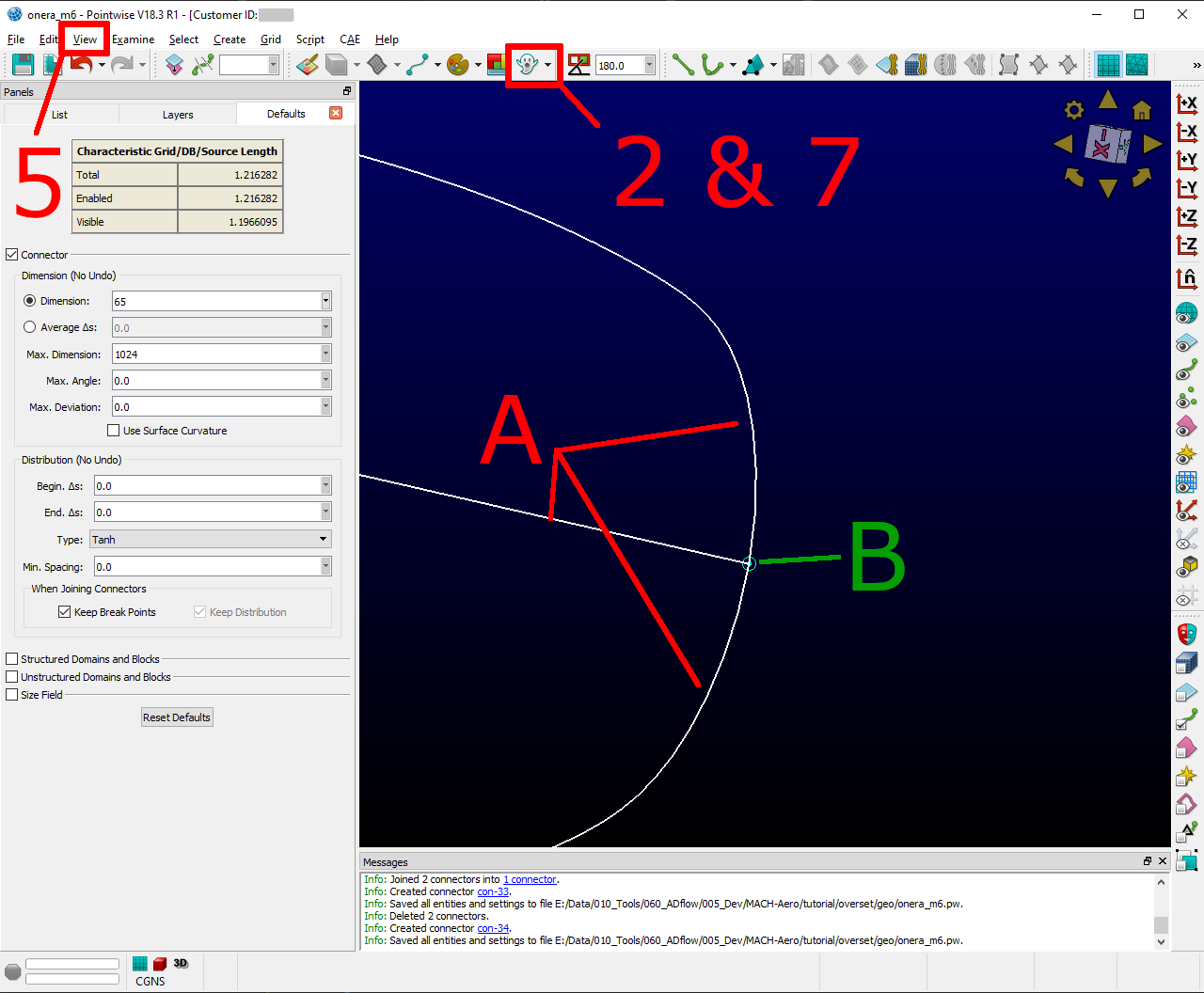
Clean up the tip LE.
Now we will dimension the remaining connectors and space the nodes properly.
Select the
3shown connectors (A)Enter
97forDimensionand hitenterClick
All Masks On/OffClick
Spacing ConstraintsSelect the
2spacing constraints at theroot LE(B)Apply
0.0008for spacingSelect the
2spacing constraints at thetip LE(C)Apply
0.0008for spacingSelect the
2spacing constraints at theroot TE(D)Apply
1.3e-5as spacingSelect the
2spacing constraints at thetip TE(E)Apply
1.3e-5as spacingSelect the
3spacing constraints at theroot(F)Apply
0.01as spacingSelect the
1spacing constraint at thetip LE(G)Apply
0.0005as spacingSelect the
2spacing constraints at thetip TE(H)Apply
1.56e-5as spacing
Apply spacing constraints for the near_tip mesh.
Next, we split the connectors at the tip to allow a topology where we can achieve a decent quality mesh.
Select the
tip topconnector (A)Click
Edit->SplitMake sure
Advancedis checkedEnter
17forIJKand hitenterClick
OKSelect the
tip bottomconnector (B)Click
Edit->Split`Enter
185forIJKand hitenterClick
OKClick on
2 Point CurvesConnect the
2newpoints(A) to (B)
Split the tip connectors.
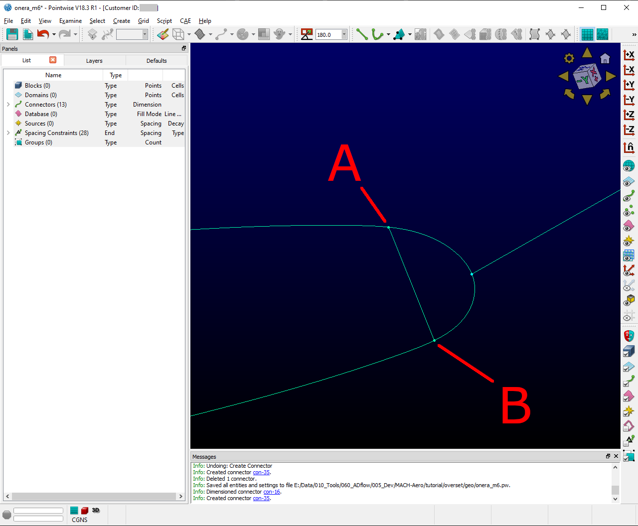
Since our tip is rounded, we have to project the newly created connector on to our database.
Select the
newlycreatedconnector(A)Click on
Edit->ProjectClick on
LayersCheck layer
0(Geo)Click on
ProjectMake sure
Target Database Selectionis checkedClick
BeginSelect the
upperandlowertip surface (hold downctrl) (B)Click
EndClick
ProjectClick
OK
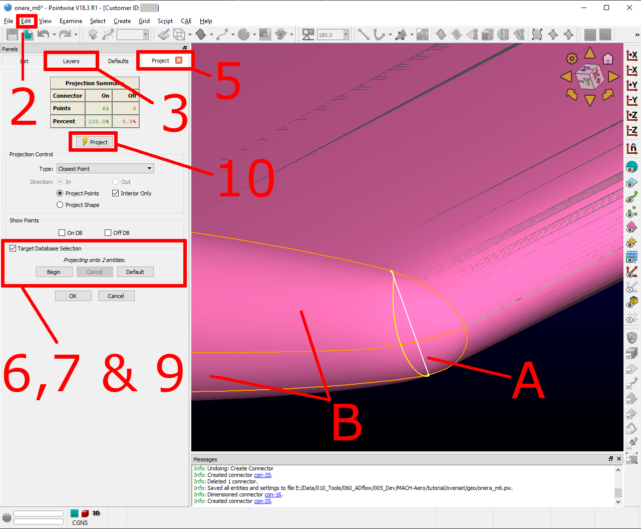
Project the connector on to the database.
Now we actually start meshing.
Click on
LayersUncheck layer
0(Geo)Select the
newlycreatedconnector(A)Click on the
arrow pointing downnext toTanh DistributionClick on
EqualClick
Edit->SplitEnter
17forIJKand hitenterEnter
49forIJKand hitenterClick
OKClick on
Create->Assemble Special->DomainSelect
1connector(B)Click
Next EdgeSelect
2connectors(C)Click
Next EdgeClick
OK
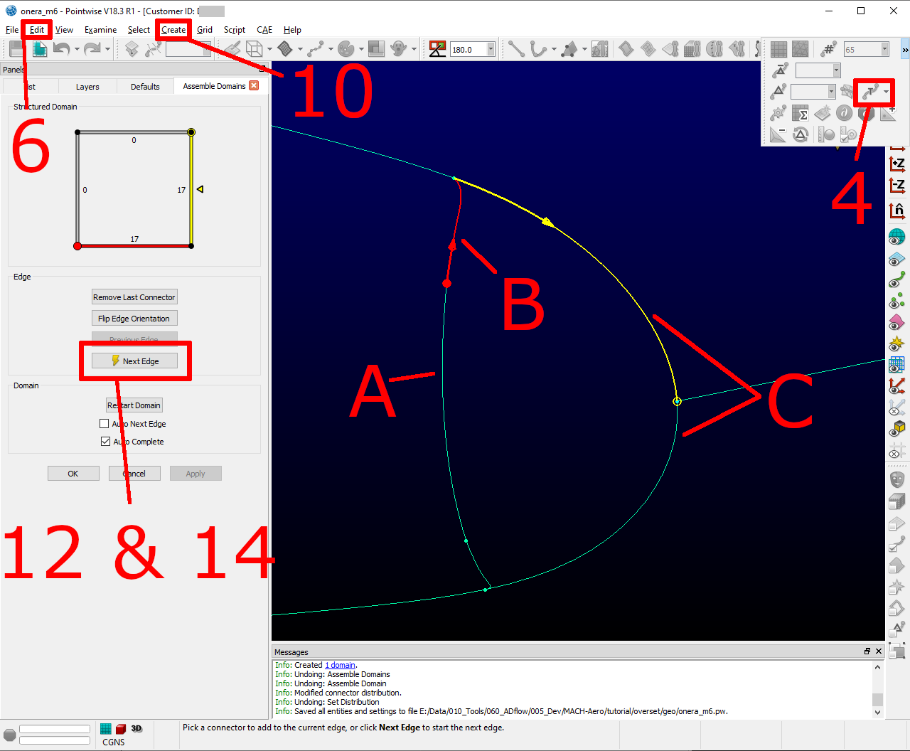
Assemble the mesh at the LE tip.
Next, we mesh the rest.
Select the
2connectors that form the semi-circle (A)Click
Script->ExecuteLook for the
scriptyou just downloaded andopenit.Select
allconnectorsClick
Assemble Domains
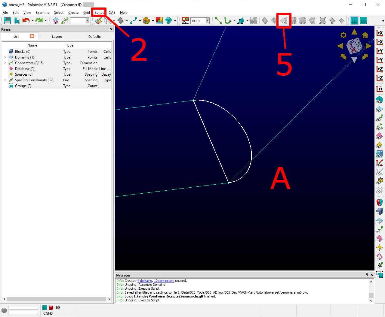
Mesh the semi-circle at the TE.
The last step is to make sure, that the skewed elements at the tip are smoothed. As Assemble Domains didn’t work
for the most outer mesh, we will delete this domain first, and create it manually again.
Select
alldomainsClick
Hidden LineSelect the
outer mostdomain and delete it (A)Select all
9connectors, that define the last remaining domainClick
Assemble DomainSelect the
newlycreateddomainand clickHidden LineSelect the
2domains that define thetip(A & B)Click
Grid->SolveClick on
Edge AttributesMake sure
Boundary Conditionsis checked and set theTypetoFloatingClick on
AttributesMake sure
Surface Shapeis checked and setShapetoDatabaseClick on
Beginand make sure, the tip is selected (it should be)Click on
EndMake sure
Solution Algorithmis checked and setSolver EnginetoSuccessive Over RelaxationSet
Relaxation FactortoNominalClick on
SolveEnter
50forIterationsand hitRunClick
OK
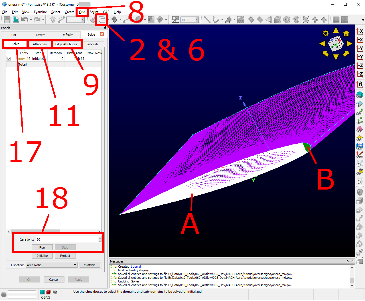
Finish the near_tip mesh.
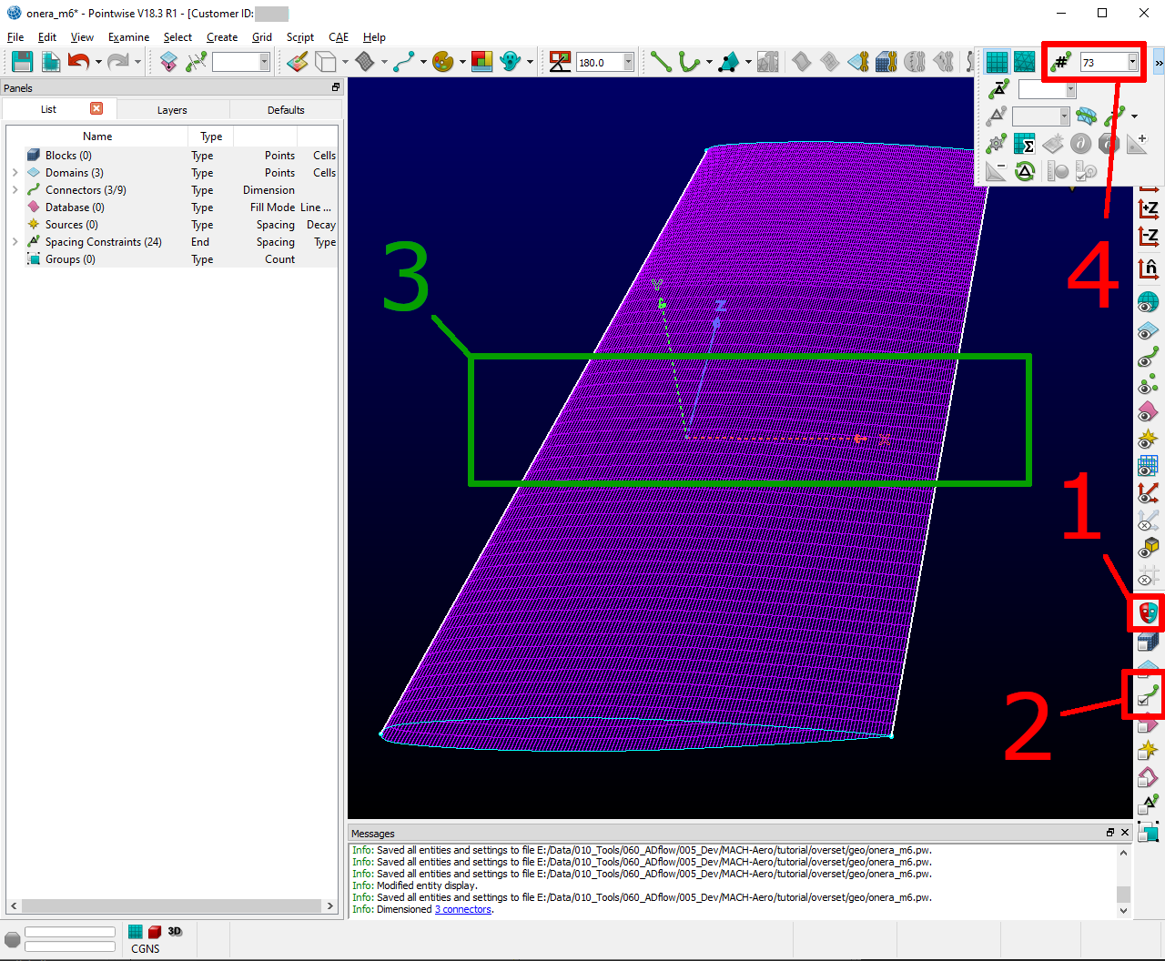
Lets check the quality of the created mesh. The most important metrics are Area Ratio and Equiangle Skewness.
Select
alldomainsClick
Examine->Area RatioClick on the
Magnification Glassnext tomaxYou see, the biggest
Area Ratiois~2.24Click on
AdvancedMake sure
HistogramandShow Histogramare checkedAs you see, the vast majority of cells has an
Area Ratioof less than1.25. This should be fineClick on
ExamineChoose
Skewness EquiangleforTypeAs you can see, the most skewed cell has a
Skewness Equiangleof~0.4. This is also fineClick
Close
Note
The lower max Area Ratio is, the easier it is to extrude a mesh with pyHyp. If it is more than 2,
it can get tricky. Skewness Equiangle describes how skewed a cell is. It should be below 0.8
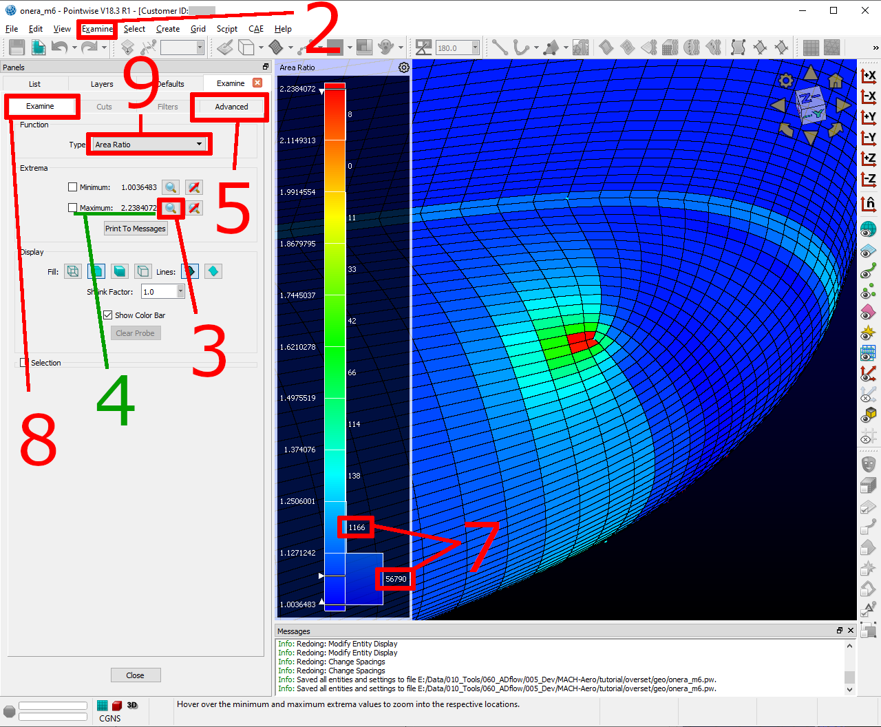
Check the mesh quality.
Export all meshes for use in pyhyp
The last step is to export the mesh. For pyHyp it is important, that the normals look in the outwards direction.
We will set the boundaries manually in pyHyp.
Note
As there has not been found an easy way to figure out which domain in Pointwise corresponds to which domain in pyHyp, it is recommended to orient them all the same way. Then apply the BC for all domains and run the pyHyp script. If an error pops up for one domain, the corresponding BC can be removed. This gets repeated until there are no errors left (This information is repeated on the next page where it probably makes more sense).
Lets start with orienting the near_tip mesh first.
Make sure only the layer
near_tipis visibleSelect
alldomainsClick
Edit->OrientSelect
onedomain (It does not matter which one)Click
I-Ja few times until you are sure, theorange arrowis pointing outwardsClick
Set MasterSelect
alldomainsClick
AlignClick
OK
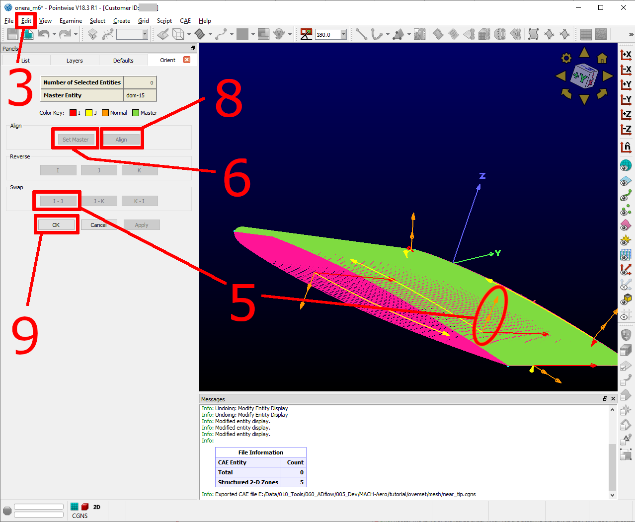
Orient the near_tip mesh so all normals point outwards.
Now we can export it.
Select
alldomainsClick
File->Export->CAESet
near_tipas Filename and save it somewhereMake sure
Data Precisionanddoubleis checkedYou can uncheck
the rest(It doesn’t really matter. But the files will be bigger if you leave it on)Press
OK
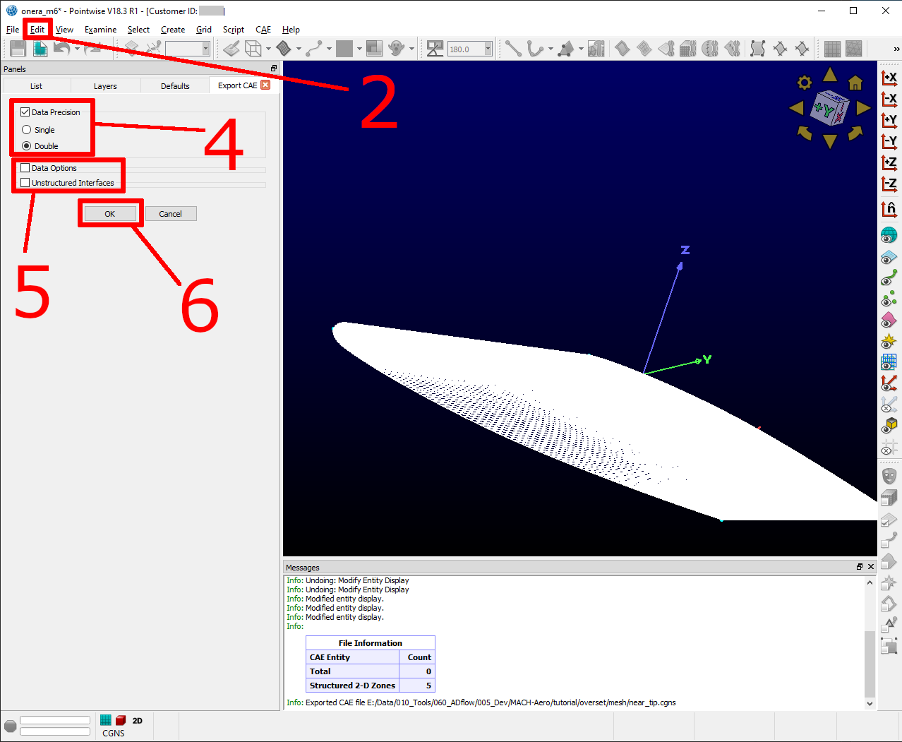
Export the near_tip mesh.
Now lets do the same for the near_wing mesh. As we have a symmetry boundary condition, the orientation
procedure is slightly more complicated.
Make sure only the layer
near_wingis visibleSelect
alldomainsClick
Edit->OrientSelect
onedomain (It doesn’t matter which one)Click
I-Juntil theorange arrowis pointing outwardsIf the
red arrowis not pointing towards the tip, clickIandI-Juntil both conditions are satisfiedClick
Set MasterSelect
alldomainsClick
AlignMake sure all
red arrowspoint towards the tip (if this is not the case, select this domain and repeat step 6)Click
OK
Now you can export the mesh near_wing like you did in the previous step.
Congratulations, you managed to create the surface mesh. On the next page, we will extrude it into a volume mesh.