CFD Analysis

Introduction

This part will help guide you through the analysis part. We will setup the run script and let ADflow compute the solution. From [O1] and [O3] we know the flow conditions:

AoA	3.06°
Mach	0.8395
Reynolds Number	11.71e6
Reynolds Ref Length	0.646m
Temperature	300° K

There is a convenience package for ADflow called adflow_util. It allows to plot the ADflow state variables live in the console and handles some annoying stuff like creating the output folder for ADflow automatically. It also makes it easy to sweep a variable, for example alpha. This utility will be used here, but the regular python API, that is detailed in other tutorials, would work as well.

For simplicity, only the calculation on the L3 mesh is covered. The other meshes might require slightly different ADflow options.

Files

Navigate to the directory overset/analysis in your tutorial folder and create an empty file called run_adflow_L3.py. If you did not create the volume mesh on the previous page, you will also have to copy the mesh file:

cp ../../../tutorial/overset/analysis/ONERA_M6_L3.cgns .

If you want to use adflow_util download and install it:

pip install git+https://github.com/DavidAnderegg/adflow_util.git

ADflow

Setup the Script

First we have to import adflow_util:

from adflow_util import ADFLOW_UTIL

Then we define a variable for the level we want to use. This makes it easier to switch, if we want to:

level = "L3"

adflow_util takes 3 different dictionaries as input. One sets some adflow_util-specific options, one sets the boundary conditions, as AeroProblem would and the last one is the regular ADflow options dict. Lets set the adflow_util options first:

options = {"name": "ONERA_M6_%s" % (level), "surfaceFamilyGroups": {"wall": ["near_wing", "near_tip"]}}

name

This sets the name for the analysis. It defines how the various output files are named.

surfaceFamilyGroups

This defines how the various surface families should be assembled. The key sets the family name and the array defines the various surfaces the family is made off.

All adflow_util options can be found here.

Now we define the AeroProblem options:

aeroOptions = {
    "alpha": 3.06,
    "mach": 0.8395,
    "reynolds": 11.72e6,
    "reynoldsLength": 0.646,
    "T": 300,
    "xRef": 0.0,
    "areaRef": 0.75750,
    "chordRef": 0.646,
    "evalFuncs": ["cl", "cd", "cmy", "cdp", "cdv"],
}

Here we set the various flow parameters. It is exactly the same as you would set in baseclasses.AeroProblem. But we could, for example, set alpha as an array of variables. In that case, adflow_util would handle everything else for us.

Now, let’s set the ADflow options:

solverOptions = {
    # Common Parameters
    "gridFile": "ONERA_M6_%s.cgns" % (level),
    "outputDirectory": "output",
    # Physics Parameters
    "equationType": "RANS",
    # RK
    "smoother": "Runge-Kutta",
    "rkreset": True,
    "nrkreset": 35,
    "CFL": 0.8,
    "MGCycle": "sg",
    "nsubiterturb": 5,
    # ANK
    "useanksolver": True,
    "anklinresmax": 0.1,
    "anksecondordswitchtol": 1e-3,
    "ankcoupledswitchtol": 1e-5,
    # NK
    "useNKSolver": True,
    "nkswitchtol": 1e-6,
    # General
    "liftindex": 3,
    "monitorvariables": ["resrho", "resturb", "cl", "cd", "yplus"],
    "printIterations": True,
    "writeSurfaceSolution": True,
    "writeVolumeSolution": True,
    "outputsurfacefamily": "wall",
    "zippersurfacefamily": "wall",
    "surfacevariables": ["cp", "vx", "vy", "vz", "blank"],
    "volumevariables": ["resrho", "rmach", "blank"],
    "nCycles": 10000,
    "L2Convergence": 1e-12,
}

Some things to note:

outputsurfacefamily

We choose wall which we defined earlier as consisting of near_wing and near_tip. This will write out only the wing as our surface solution.

zippersurfacefamily

This tells ADflow which surfaces it should use to construct the geometry on which the forces are integrated.

surfacevariables & volumevariables

Here it is very important to add blank. This way we know which cells we can hide in the postprocessor as the ‘blanked’ cells still show up in the solution.

Note

To only view computed cells, add a filter to your post-processor in a way, that only cells where blank is bigger than 0 are shown.

And lastly, we plug everything into adflow_util:

au = ADFLOW_UTIL(aeroOptions, solverOptions, options)
au.run()

Simply Run the Script

To run the script, proceed as usual:

python run_adflow_L3.py

If you want to run in parallel, start it with MPI:

mpirun -np 4 python run_adflow_L3.py

Plot the Iterations in realtime

If you want to have a graphical representation of all the ADflow variables, adflow_util comes in handy as well. It has an additional package called adflow_plot. If you installed it using pip, you can simply start it this way:

adflow_plot -i run_adflow_L3.py

If you want to run in parallel:

adflow_plot -i run_adflow_L3.py -np 4

This is simply an overlay, which starts the adflow script in the background and parses it’s stdout. At startup you will see the regular adflow-ouput. But as soon as the calculation starts, you’ll see a plot of resRho:

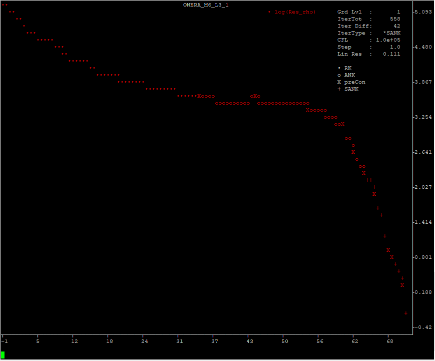
adflow_plot output.

At the bottom is a console where you can define which variables you want to see. As terminals usually have a low number of ‘pixels’, it is also possible to show only a limited number of iterations. Simply type help or h and hit Enter. You will get a list of all available commands. To quit, simply type q and confirm with y.

Output files

In addition to the expected volume and surface files from adflow, there will also be a file called ONERA_M6_L3.out. It is from adflow_util and looks like this:

ONERA_M6_L3

Aero Options
--------------  ---------------------
alpha           3.06
mach            0.8395
reynolds        11720000.0
reynoldsLength  0.646
T               300
xRef            0.0
areaRef         0.7575
chordRef        0.646
evalFuncs       cl, cd, cmy, cdp, cdv
--------------  ---------------------


RESULTS
        cd         cdp         cdv          cl          cmy    totalRes    iterTot
----------  ----------  ----------  ----------  -----------  ----------  ---------
0.01879813  0.01326940  0.00552873  0.26064807  -0.18639411  0.00011945         82

It gives us a nice summary of the input and output values. If we had a sweep variable defined, the multiple points would be listed here too.

Results

For validation purposes, ADflow was run with all meshes and the results were plotted against various different solvers from [O3]. As you can see, ADflow lies right in the middle:

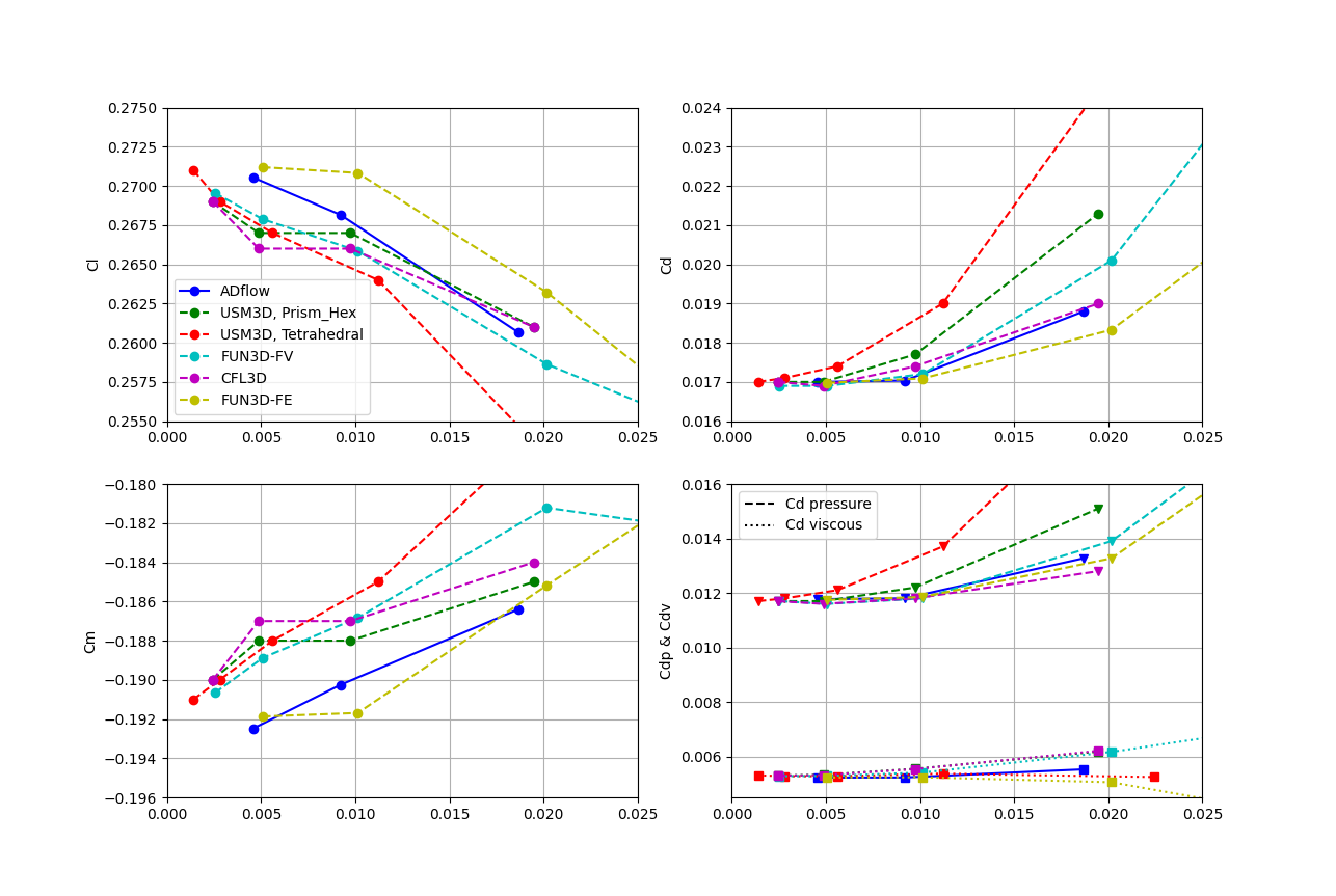
Grid Convergence of ADflow in comparison to various other solvers.