Overview of MACH-Aero
This page provides an overview of the aerodynamic shape optimization capability within MACH (framework for MDO of aircraft configurations with high fidelity).
MACH-Aero consists of six major modules:
Pre-processing (pyHyp, ANSYS ICEM-CFD)
Geometry parameterization (pyGeo)
Volume mesh deformation (IDWarp)
Optimization (pyOptSparse)
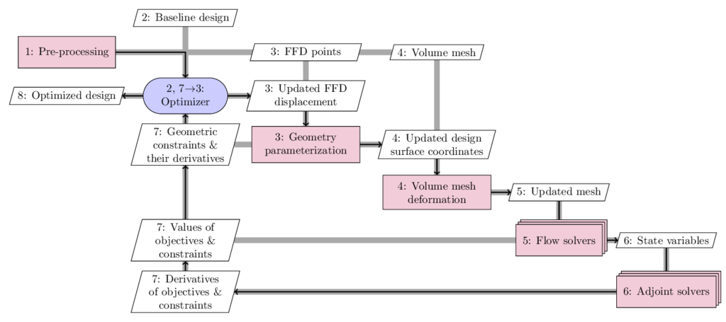
Generally, MACH-Aero starts with a baseline design and uses the gradient to find the most promising direction in the design space for improvement. This process is repeated until the optimality and feasibility conditions are satisfied. More specifically, the process is as follows, using the above figure as a reference. Here we use the extended design structure matrix (XDSM) representation developed by Lambe and Martins (2012). The diagonal nodes represent the modules and the off-diagonal nodes represent the data. The black lines represent the process flow for the adjoint solver, whereas the thick gray lines represent the data flow. The number in each node represents the execution order:
First, we generate a volume mesh for the baseline geometry (pre-processing in process 1). Several mesh generation tools are available including pyHyp and ICEM. Refer to Surface Meshing, Volume Meshing, and Mesh Manipulation for more details. The generated mesh will be used later in process 4. In the pre-processing step, we also generate free-form deformation (FFD) points (process 3) that will be used later to morph the design surface. Refer to Geometric Parameterization.
Then, we give a set of baseline design variables to the optimizer (process 2). We usually use SNOPT as the optimizer, which uses the SQP algorithm. We use pyOptSparse to facilitate the optimization problem setup. The optimizer will update the design variables and give them to the geometry parameterization module (pyGeo; process 3). pyGeo receives the updated design variables and the FFD points generated in the pre-processing step, performs the deformation for the design surface, and outputs the deformed design surface to the mesh deformation module (IDWarp) in process 4. pyGeo also computes the values of geometric constraints and their derivatives with respect to the design variables (process 7).
Next, IDWarp deforms the volume mesh based on the updated design surface and outputs the updated volume mesh to the flow simulation module in process 5.
The flow simulation module receives the updated volume mesh and uses high-fidelity CFD tools (i.e., ADflow or DAFoam) to compute the state variables (process 6) or physical fields (pressure, density, velocity, etc.). The flow simulation module also computes the objective and constraint functions (e.g., drag and lift; see process 7) and outputs the state variables to the adjoint computation module.
Then, the adjoint computation module (process 6) computes the total derivatives of the objective and constraint functions with respect to the design variables (process 7) and gives them back to the optimizer in process 7. The benefit of using the adjoint method to compute derivatives is that its computational cost is independent of the number of design variables, which makes it attractive for handling large-scale, complex design problems such as aircraft design. There are two available adjoint solvers: ADflow, DAFoam.
Finally, the optimizer receives the values and derivatives of the objective and constraint functions in process 7, performs the SQP computation, and outputs a set of updated design variables to pyGeo.
The above process is repeated until the optimization converges. Refer to the MACH-Aero tutorials for tutorials.