Volume Meshing
Introduction
The objective of this section is to create a family of volume meshes using pyHyp. We previously used pyHyp to extrude our airfoil coordinates into a volume mesh. However, this time we will use it to extrude our surface mesh coordinates into a volume mesh. The surface mesh serves as the seed for hyperbolically marching the mesh to the farfield. Generating the volume mesh in this way is fast, repeatable, and results in a high-quality mesh. We will take advantage of the surface mesh coarsening features to generate a family of volume meshes. Additionally, we will demonstrate a few additional settings in pyHyp compared to what was shown in the airfoil tutorial.
Files
Navigate to the directory wing/meshing/volume in your tutorial folder.
Create the following empty runscript in the current directory:
run_pyhyp.py
Dissecting the pyHyp runscript
Open the file run_pyhyp.py with your favorite text editor.
Then copy the code from each of the following sections into this file.
Import libraries
import argparse
from pyhyp import pyHyp

parser = argparse.ArgumentParser()
parser.add_argument("--level", default="L3")
args = parser.parse_args()
This is the standard way of importing the pyHyp library. We also import the argument parser and setup it up to allow us to specify which level of mesh we want to extrude.
Setup parameters for each member of the mesh family
if args.level in ["L0.5", "L1.5", "L2", "L3", "L4"]:
    family = args.level
else:
    family = "L1"

coarsen_levels = {
    "L0.5": 1,
    "L1": 1,
    "L1.5": 2,
    "L2": 2,
    "L3": 3,  # debug only level
    "L4": 4,  # debug only level
}
coarsen = coarsen_levels[args.level]

ngrid_levels = {
    "L0.5": 257,
    "L1": 193,
    "L1.5": 129,
    "L2": 97,
    "L3": 49,
    "L4": 37,
}
ngrid = ngrid_levels[args.level]

level_fact = {
    "L0.5": 4 * 1.414,
    "L1": 4.0,
    "L1.5": 2.0 * 1.414,
    "L2": 2.0,
    "L3": 1.0,
    "L4": 0.5,
}
s0 = 1e-5 / level_fact[args.level]
We want to create a family of meshes with the L3 mesh being the coarsest and the L0.5 mesh being the finest. In between we want an L2, L1.5, and L1 mesh. Here we are goint to parse our input argument to determine which level of refinment we will generate on this run. We default to L1 if the argument is invalid or no argument is provided. Using the specified level of refinement we select the amount of surface mesh coarsening we will use, the number of off wall layers to extrude too, and the initial off wall spacing from a list.
Options
options = {
    # ---------------------------
    #   General options
    # ---------------------------
    "inputFile": "../surface/wing_surf_L1.cgns",
    "fileType": "CGNS",
    "unattachedEdgesAreSymmetry": True,
    "outerFaceBC": "farfield",
    "autoConnect": True,
    "BC": {},
    "families": "wall",
Just like before we need to pass a dictionary of options to pyHyp for mesh extrusion. Note that this time the options we use are a little different and that we need to take advantage for a few more options for a family of wing meshes. A complete list of definitions of the pyHyp options can be found in the pyHyp documentation. Here we will point a few more of the options.
General options:
inputFileName of the surface mesh file.
fileTypeFiletype of the surface mesh file. Either
cgnsorplot3d.unattachedEdgesAreSymmetryTells pyHyp to automatically apply symmetry boundary conditions to any unattached edges (those that do not interface with another block).
outerFaceBCTells pyHyp to which boundary condition to apply to the outermost face of the extruded mesh. Either
farfieldoroverset.familiesName given to wall surfaces. If a dictionary is submitted, each wall patch can have a different name. This can help the user to apply certain operations to specific wall patches in ADflow.
    # ---------------------------
    #   Grid Parameters
    # ---------------------------
    "coarsen": coarsen,
    "N": ngrid,
    "s0": s0,
    "marchDist": 23.2 * 14,
- Grid parameters:
coarsenAutomatically coarsen the surface mesh before starting extrusion.
1gives the same surface mesh.2coarsens by a factor of 2 in each direction.3coarsens by a factor of 4 in each direction, and so on. Here will will pass in the value we selected from the list above for our specific mesh refinement level.NNumber of nodes in off-wall direction. Here will will pass in the value we selected from the list above for our specific mesh refinement level. If multigrid will be used this number should be 2m-1 (n+1), where m is the number of multigrid levels and n is the number of layers on the coarsest mesh.
s0Thickness of first off-wall cell layer. Here will will pass in the value we selected from the list above for our specific mesh refinement level.
marchDistDistance of the far-field.
The following options are related to the algorithms that are used to generate the mesh and usually these default values do not need to be modified.
More information can be found in the pyHyp documentation.
For example, epsE may be of interest when dealing with concave corners.
One thing to note there is that we have applied something called scheduleing to some of these parameters.
This is when we don’t just pass a single value but a list of value pairs where the second term is the value of the parameter and the first is the point (as a fraction) in the mesh extrusion process it should be applied.
    # ---------------------------
    #   Pseudo Grid Parameters
    # ---------------------------
    "ps0": -1.0,
    "pGridRatio": -1.0,
    "cMax": 1.0,
    # ---------------------------
    #   Smoothing parameters
    # ---------------------------
    "theta": 3.0,
    "volCoef": 0.25,
    # apply scheduling to all grids
    "volSmoothiter": [[0.0, 20], [0.3, 50], [0.7, 100], [1.0, 100]],
    "volBlend": [[0.0, 1e-6], [0.5, 1e-6], [0.8, 1e-4], [1.0, 1e-3]],
    "epsE": [[0.0, 0.5], [0.5, 1.0], [0.9, 2.0], [1.0, 4.0]],
    "epsI": [[0.0, 1.0], [0.5, 2.0], [0.9, 4.0], [1.0, 8.0]],
    # ---------------------------
    #   Solution Parameters
    # ---------------------------
    "kspRelTol": 1e-8,
    "kspMaxIts": 1500,
    "kspSubspaceSize": 50,
}
Running pyHyp is quite simple, as shown below.
After the mesh extrusion is done, we can write the volume mesh with the writeCGNS function.
hyp = pyHyp(options=options)
hyp.run()
hyp.writeCGNS(f"wing_vol_{args.level}.cgns")
Note
Be mindful of the growth ratio When extruding the mesh the growth ratio is a key parameter to pay attention to. It’s defined as the the ratio of the length in offwall direction of the cells in a particular layer over the length in the offwall direction of the cells in the previous layer. Changing the the number of layers without the changing the march distance or initial offwall cell size will change the growth ratio. A growth ratio of 1.3 is recommended for these cases presented in these tutorials. pyHyp does support a parameter for setting the growth ratio manually but this will ignore the set march distance so it’s not often used.
Run it yourself!
When running you will need to specify which refinement level you want to generate. For this tutorial having a L3, L2, and L1 mesh is sufficient but feel free to generate others. You can now run the python file with the command:
python run_pyhyp.py --level {insert refinement level here}
For larger meshes, you will want to run pyHyp as a parallel process. This can be done with the command:
mpiexec -n 4 python run_pyhyp.py --level {insert refinement level here}
where the number of processors is given after -np.
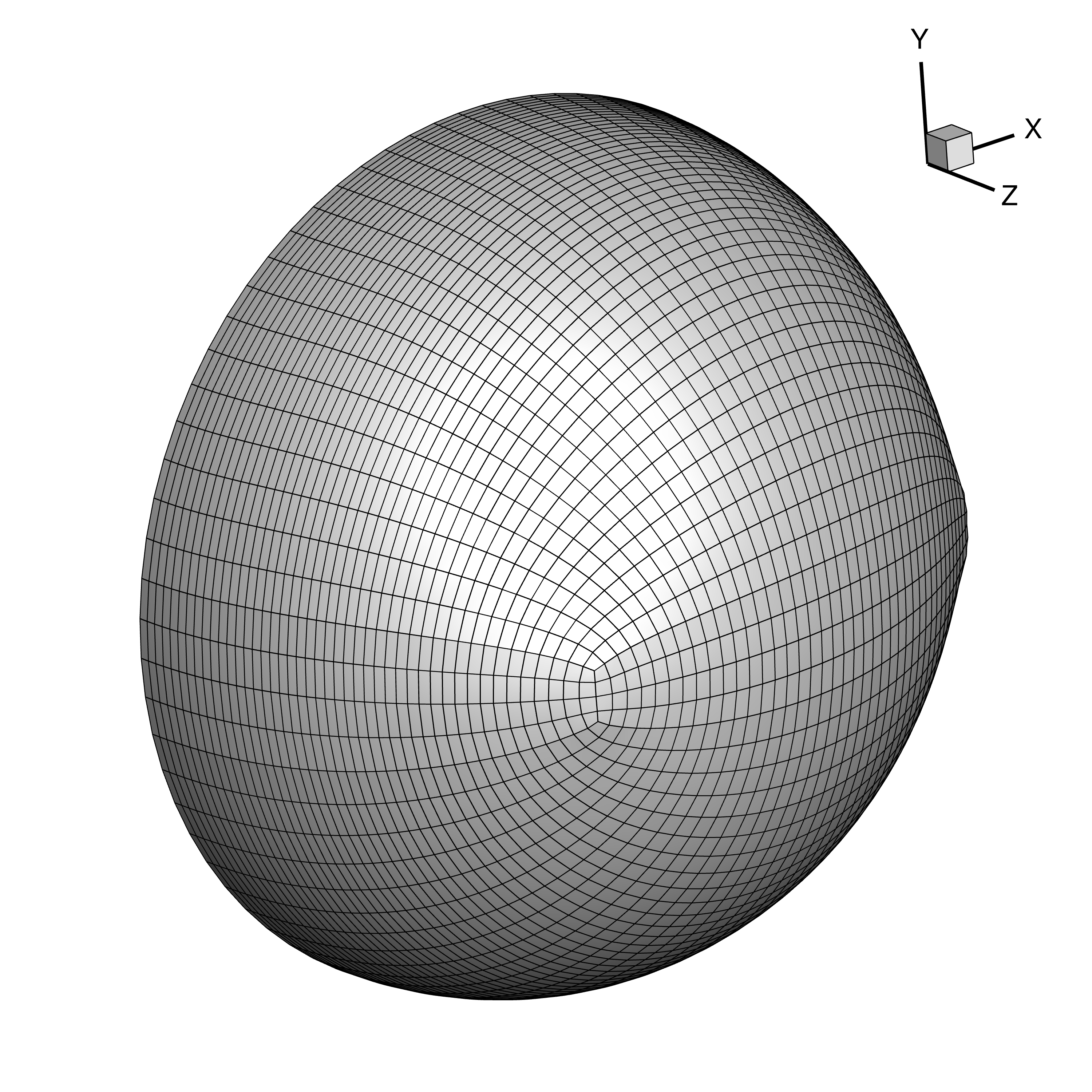
You can open wing_vol_{refine level}.cgns in Tecplot to view the volume mesh.
The output should look similar to the image below.