Grid Refinement Study
Theory
Computational physics models generally use discretized physical domains (grids) to transform physical laws into systems of equations that can be solved by numerical methods. The discretization of a physical domain introduces discretization error, which can be reduced in two ways:
- \(h\)-refinement
Increasing the resolution of the grid.
- \(p\)-refinement
Increasing the order of the numerical approximation at each cell.
In a grid refinement study, we demonstrate that iterative h-refinement converges to the exact solution. For a given grid/mesh, the grid spacing is
where \(N\) is the number of cells and \(d\) is the dimension of the domain. For two grids, the grid refinement ratio is
Generally, we use a grid refinement ratio of 2. The convention is to name the grids with an L (for level) followed by an integer beginning at 0 for the finest grid (i.e. L0 for the finest, L1 for the next, etc).
If the grids are sufficiently fine, the error is roughly proportional to \(h^p\), where \(p\) is the order of the solution method. Grids that follow this relationship are in what is termed the “region of asymptotic convergence”. Although for a second-order finite volume solver, the theoretical order of convergence is \(p=2\), the achieved rate of convergence (\(\hat{p}\)) may vary. The achieved rate of convergence for a given h-refinement study can be computed as
using the finest three grids. When plotting the results of the grid convergence study, we generally plot the results of the grid convergence using \(h^p\) on the x-axis.
The Richardson extrapolation is an estimation of the solution for a grid with a grid spacing on the order of zero. It is computed using the solutions from the L0 and L1 grids with the equation
Approaches to Grid Refinement
There are two methods we use for performing grid refinement:
coarsening the volume mesh or
coarsening the surface mesh and extruding the family of surface meshes.
We discuss the pros and cons of each method and underlying theory; it is up to the user to choose the method.
A few general notes first:
The bottom line is as long as the CFD mesh is fine enough to capture the correct physical trends, then the design space will be accurate enough such that coarse mesh optimizations will get you close enough to the optimal solution. Subsequently, one can use finer meshes using the design variables from the coarser optimizations, thus decreasing overall computational cost.
Redo your mesh convergence study on the optimized result to double check everything is behaving as expected
Plotting contours of \(y^+\) can help with debugging
This whole refinement study is also not as simple with a coupled structural model because, depending on the structural model, there are likely differences in order of the method (TACS has linear finite elements) and truncation error constants, all of which will affect the observed order of accuracy.
Option 1: Coarsening volume meshes
Generate a fine grid (L0) with \(N=(2^n) (m) + 1\) nodes along each edge.
Coarsen the L0 grid \(n-1\) times using
cgns_utils coarsen.Compute the Richardson extrapolation using the L0 and L1 grid solutions.
Plot \(h^p\) vs \(C_D\). For ADflow, start by assuming \(p=2\).
This mesh refinement method is consistent with the original Richardson extrapolation theory, which relies on uniform coarsening between meshes. A mesh is in the asymptotic range if it lies on the line connecting the extrapolated value and the finest mesh value. If you do not get this despite using fine meshes, this usually means the output you are looking at is not second-order accurate (which is rather common). In this case, redo the extrapolation after determining the achieved rate of convergence as described in Theory. The slope of the line is the coefficient of the leading truncation error term.
An example of grid convergence plot for a family of RAE 2822 Airfoil meshes is illustrated below:
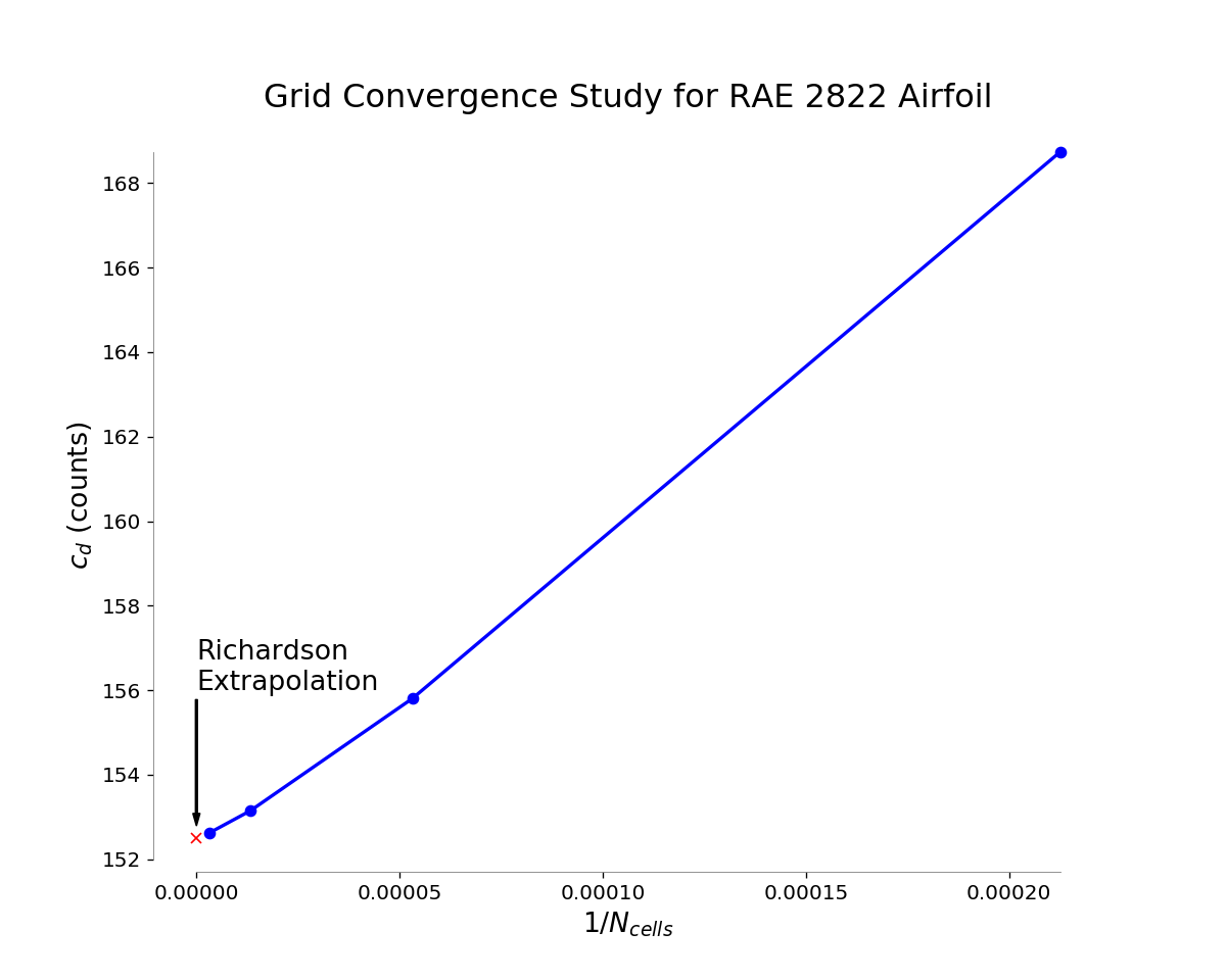
Figure 1: Grid convergence plot for RAE 2822 Transonic Airfoil.
- Pros:
The grid is coarsened uniformly, giving the most mathematically rigorous convergence study, which is important for justifying solutions in your scholarly articles.
- Cons:
For 3D meshes, the finest mesh (L0) has to be extremely fine for the L2 mesh to still be in the asymptotic regime. This is because the \(n\)th level will have \(2^{3n}\) fewer cells for a refinement ratio of 2. This can be a problem if you want to conduct a refinement study using the L0, L1, and L2 meshes.
The growth ratios change, so be wary of the off-wall cell resolution and boundary layer accuracy.
Option 2: Coarsening surface meshes and extruding a family of volume meshes
An alternative to using cgns_utils coarsen is to coarsen the surface mesh and re-extrude the volume meshes.
The main motivation for this is to generate meshes without changing the growth rate of the off-wall layers.
In addition, node clustering in all directions is better with this method.
If you use cgns_utils coarsen (i.e. Option 1: Coarsening volume meshes), you will be able to increase the first off-wall spacing s0 uniformly.
However, the growth ratio is going to change, and the off-wall layers may have too much distance between each other.
For airfoils, we can use the prefoil package to coarsen or refine the surface meshes.
An example script is given below.
You can either provide a .dat file or create the NACA 4 digit airfoils.
Then, you can manipulate the meshing parameters and get different mesh levels.
from pyhyp import pyHyp
from prefoil import sampling, Airfoil
from prefoil.utils import generateNACA


# L2 layer mesh grid initilization
# We will refine the mesh from this starting grid
nTE_cells_L2 = 5
nSurfPts_L2 = 200
nLayers_L2 = 80
s0_L2 = 4e-6

# Increasing the mesh sizes
refinement = [1, 2, 4]
level = ["L2", "L1", "L0"]

for i in range(len(refinement)):
    # number of points on the airfoil surface
    nSurfPts = refinement[i] * nSurfPts_L2

    # number of points on the TE.
    nTEPts = refinement[i] * nTE_cells_L2

    # number of extrusion layers
    nExtPts = refinement[i] * nLayers_L2

    # first off wall spacing
    s0 = s0_L2 / refinement[i]

    #### We can either import our desired airfoil .dat file and continue the meshing proces ####
    #### Or we can generate the NACA airfoils if our baseline is a 4 series NACA airfoil    ####

    # We can also  generate NACA 4 series airfoils
    code = "0012"
    nPts = 150
    initCoords = generateNACA(code, nPts, spacingFunc=sampling.polynomial, func_args={"order": 8})
    airfoil = Airfoil(initCoords)

    coords = airfoil.getSampledPts(
        nSurfPts,
        spacingFunc=sampling.polynomial,
        func_args={"order": 8},
        nTEPts=nTEPts,
    )

    # Write surface mesh
    airfoil.writeCoords(f"./input/naca0012_{level[i]}", file_format="plot3d")

    options = {
        # ---------------------------
        #        Input Parameters
        # ---------------------------
        "inputFile": f"./input/naca0012_{level[i]}.xyz",
        "unattachedEdgesAreSymmetry": False,
        "outerFaceBC": "farfield",
        "autoConnect": True,
        "BC": {1: {"jLow": "zSymm", "jHigh": "zSymm"}},
        "families": "wall",
        # ---------------------------m
        #        Grid Parameters
        # ---------------------------
        "N": nExtPts,
        "s0": s0,
        "marchDist": 100.0,
    }

    hyp = pyHyp(options=options)
    hyp.run()
    hyp.writeCGNS(f"./input/naca0012_{level[i]}.cgns")
The figure below shows a comparison between coarsening a mesh with cgns_utils and prefoil.
When we coarsen with cgns_utils, the distance between each layer is higher and the growth ratio is not the same as the prefoil mesh.
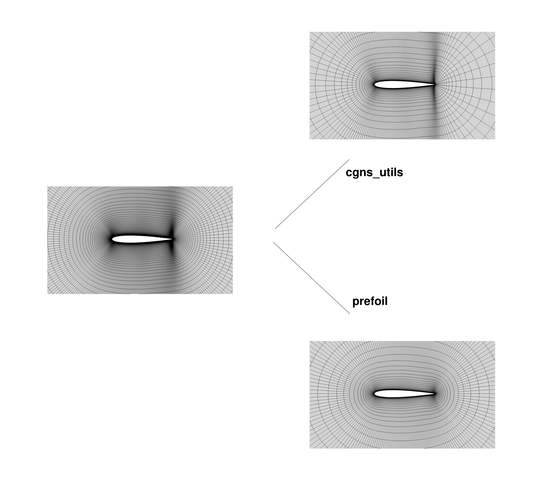
Figure 2: Mesh comparison.
For 3D, you will have to modify the surface mesh discretization in your meshing software (e.g., ICEM/Pointwise).
- Pros:
It is more practical for 3D meshes because you can use a less aggressive refinement ratio compared to
Option 1(i.e., \(r < 2\)). This places the points on the refinement plot closer to each other on the \(x\)-axis, so it is more likely that your coarsest volume mesh is in the asymptotic regime, which you can then use for coarse optimizations.It is the only way to generate the 0.5 level family of meshes (e.g., L0.5, L1.5, L2.5) using the
scaleBlkFileprocedure in the postprocessing repository to scale the surface meshes by a factor of \(1/\sqrt{2}\).
- Cons:
It is harder to be mathematically rigorous (and therefore justifiable in a scholarly article) using this method because all options from the surface mesh extrusion have to be scaled accordingly, and even then, there may be variations in volume cell scaling from the procedure.
Your mesh refinement results might not follow a perfectly straight line compared to
Option 1even if they are in the asymptotic regime since it is not a uniform refinement (but it should be close to linear). Improper scaling of the off-wall and far-field cells may add to discretization error.