Single Point Optimization

Introduction

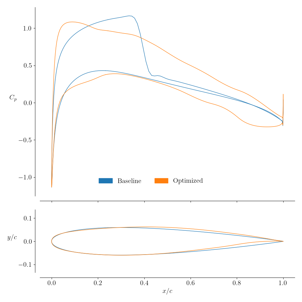
We will now proceed to optimizing a NACA0012 airfoil for a given set of flow conditions. The optimization problem is defined as:

minimize

\(C_D\)

with respect to

10 shape variables

subject to

\(C_L = 0.5\)
\(V \ge V_0\)
\(t \ge 0.1t_0\)
\(\Delta z_\text{LETE, upper} = -\Delta z_{LETE, lower}\)

The shape variables are controlled by the FFD points specified in the FFD file.

Files

Navigate to the directory airfoilopt/singlepoint in your tutorial folder. Create the following empty runscript in the current directory:

airfoil_opt.py

Dissecting the aerodynamic optimization script

Open the file airfoil_opt.py in your favorite text editor. Then copy the code from each of the following sections into this file.

Import libraries

import os
import numpy as np
import argparse
import ast
from mpi4py import MPI
from baseclasses import AeroProblem
from adflow import ADFLOW
from pygeo import DVGeometry, DVConstraints
from pyoptsparse import Optimization, OPT
from idwarp import USMesh
from multipoint import multiPointSparse

Adding command line arguments

# Use Python's built-in Argument parser to get commandline options
parser = argparse.ArgumentParser()
parser.add_argument("--output", type=str, default="output")
parser.add_argument("--opt", type=str, default="SLSQP", choices=["SLSQP", "SNOPT"])
parser.add_argument("--gridFile", type=str, default="../../airfoil/meshing/n0012.cgns")
parser.add_argument("--optOptions", type=ast.literal_eval, default={}, help="additional optimizer options to be added")
args = parser.parse_args()

This is a convenience feature that allows the user to pass in command line arguments to the script. Four options are provided:

Output directory
Optimizer to be used
Grid file to be used
Optimizer options

Specifying parameters for the optimization

# cL constraint
mycl = 0.5
# angle of attack
alpha = 1.5
# mach number
mach = 0.75
# cruising altitude
alt = 10000

Several conditions for the optimization are specified at the beginning of the script. These include the coefficient of lift constraint value, Mach number, and altitude to indicate flow conditions. The angle of attack serves as the initial value for the optimization and should not affect the optimized result.

Creating processor sets

MP = multiPointSparse(MPI.COMM_WORLD)
MP.addProcessorSet("cruise", nMembers=1, memberSizes=MPI.COMM_WORLD.size)
comm, setComm, setFlags, groupFlags, ptID = MP.createCommunicators()
if not os.path.exists(args.output):
    if comm.rank == 0:
        os.mkdir(args.output)

Allocating sets of processors for different analyses can be helpful for multiple design points, but this is a single-point optimization, so only one point is added.

ADflow options

aeroOptions = {
    # Common Parameters
    "gridFile": args.gridFile,
    "outputDirectory": args.output,
    "monitorvariables": ["resrho", "cl", "cd"],
    "writeSurfaceSolution": False,
    "writeVolumeSolution": False,
    # Physics Parameters
    "equationType": "RANS",
    # Solver Parameters
    "smoother": "DADI",
    "MGCycle": "sg",
    "nSubiterTurb": 10,
    "liftIndex": 2,
    "infChangeCorrection": True,
    # ANK Solver Parameters
    "useANKSolver": True,
    # NK Solver Parameters
    "useNKSolver": True,
    "NKSubSpaceSize": 400,
    "NKASMOverlap": 4,
    "NKPCILUFill": 4,
    "NKJacobianLag": 5,
    "NKSwitchTol": 1e-6,
    "NKOuterPreConIts": 3,
    "NKInnerPreConIts": 3,
    # Convergence Parameters
    "L2Convergence": 1e-15,
    "L2ConvergenceCoarse": 1e-4,
    "nCycles": 20000,
    # Adjoint Parameters
    "adjointSolver": "GMRES",
    "adjointL2Convergence": 1e-12,
    "ADPC": True,
    "adjointMaxIter": 5000,
    "adjointSubspaceSize": 100,
    "ILUFill": 3,
    "ASMOverlap": 3,
    "outerPreconIts": 3,
    "frozenTurbulence": False,
    "restartADjoint": False,
}

# Create solver
CFDSolver = ADFLOW(options=aeroOptions, comm=comm)

# Create slice
span = 1.0
pos = np.array([0.5]) * span
CFDSolver.addSlices("z", pos, sliceType="absolute")

In this example, we have configured far more options for ADflow than we did in the previous example. For optimziation problems, the solver needs to be tuned for high performance and robustness. As it is, the options specified above allow for a good convergence of NACA0012 airfoil analysis, but may not converge for other airfoils. We won’t go over all the options and why we selected them here but will refer you to the ADflow documentation. However some useful options to adjust are:

nCycles: If the analysis doesn’t converge, this can be increased.
NKSwitchTol: If the analysis stops converging during NK (Newton-Krylov), this might mean that it is still outside of the radius of convergence of the NK method. The parameter should then be lowered.
NKSubSpaceSize: Decreasing this parameter will decrease memory usage when in the NK solver. Only change this if there are memory issues when dealing with larger meshes.
writeSurfaceSolution and writeVolumeSolution: If you want to view the surface or volume solutions at the end of each analysis, these parameters can be set to True.

We then create the ADflow solver object while passing in the options dictionary and communicator object. We also use addSlices to write the airfoil coordinates and \(c_p\) distribution to a text file.

Set the AeroProblem

ap = AeroProblem(name="fc", alpha=alpha, mach=mach, altitude=alt, areaRef=1.0, chordRef=1.0, evalFuncs=["cl", "cd"])
# Add angle of attack variable
ap.addDV("alpha", value=alpha, lower=0, upper=10.0, scale=1.0)

We add angle of attack as a design variable and set up the AeroProblem using given flow conditions.

Geometric parametrization

# Create DVGeometry object
FFDFile = "../ffd/ffd.xyz"

DVGeo = DVGeometry(FFDFile)
DVGeo.addLocalDV("shape", lower=-0.05, upper=0.05, axis="y", scale=1.0)

# Add DVGeo object to CFD solver
CFDSolver.setDVGeo(DVGeo)

The set-up for DVGeometry (FFD class) is simple for an airfoil since it doesn’t involve span-wise variables such as twist, dihedral, or taper. The only DVs we have are local shape variables that control the vertical movements of each individual FFD node. The local design variable shape is added.

Note

Note that since we have to work with a 3D problem, this in fact has twice as many DVs as we’d like—the shape of the two airfoil sections should remain the same. This is addressed by adding linear constraints in the following section.

Geometric constraints

DVCon = DVConstraints()
DVCon.setDVGeo(DVGeo)

# Only ADflow has the getTriangulatedSurface Function
DVCon.setSurface(CFDSolver.getTriangulatedMeshSurface())

le = 0.0001
leList = [[le, 0, le], [le, 0, 1.0 - le]]
teList = [[1.0 - le, 0, le], [1.0 - le, 0, 1.0 - le]]

DVCon.addVolumeConstraint(leList, teList, 2, 100, lower=1, scaled=True)
DVCon.addThicknessConstraints2D(leList, teList, 2, 100, lower=0.1, upper=3.0)

DVConstraints is the class in pygeo responsible for handling geometric constriants. There are several built-in constraint functions within the DVConstraints class, including thickness, surface area, volume, location, and general linear constraints. The majority of the constraints are defined based on a triangulated-surface representation of the airfoil obtained from ADflow.

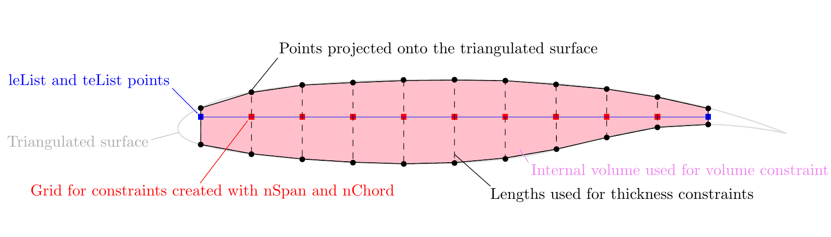
The two primary geometric constraints of interest in our optimization problem are the thickness and area of the airfoil. We can address both these constraints by using the addThicknessConstraints2D function for the thickness constraints and the addVolumeConstraint for area (remember the airfoil is a one cell thick 3D object). The volume and thickness constraints are set up by creating a uniformly spaced 2D grid of points, which is then projected onto the upper and lower surface of a triangulated-surface representation of the airfoil. The grid is defined by providing four corner points (using leList and teList) and by specifying the number of spanwise and chordwise points (using nSpan and nChord). Remember that we are treating the airfoil as the one cell deep 3D object so it technically has a “span”. By default, scaled=True for addVolumeConstraint() and addThicknessConstraints2D(), which means that the volume and thicknesses calculated will be scaled by the initial values (i.e., they will be normalized). Therefore, lower=1.0 in this example means that the lower limits for these constraints are the initial values (i.e., if lower=0.5 then the lower limits would be half the initial volume and thicknesses).

For the volume constraint, the volume is computed by adding up the volumes of the prisms that make up the projected grid as illustrated in the following image. For the thickness constraints, the distances between the upper and lower projected points are used, as illustrated in the following image. During optimization, these projected points are also moved by the FFD, just like the airfoil surface, and are used again to calculate the thicknesses and volume for the new designs. More information on the options can be found in the pyGeo docs or by looking at the pyGeo source code.

../_images/opt_thickness_and_vol_diagram.png

Warning

The leList and teList points must lie completely inside the airfoiil.

# Le/Te constraints
lIndex = DVGeo.getLocalIndex(0)
indSetA = []
indSetB = []
for k in range(0, 1):
    indSetA.append(lIndex[0, 0, k])  # all DV for upper and lower should be same but different sign
    indSetB.append(lIndex[0, 1, k])
for k in range(0, 1):
    indSetA.append(lIndex[-1, 0, k])
    indSetB.append(lIndex[-1, 1, k])
DVCon.addLeTeConstraints(0, indSetA=indSetA, indSetB=indSetB)

# DV should be same along spanwise
lIndex = DVGeo.getLocalIndex(0)
indSetA = []
indSetB = []
for i in range(lIndex.shape[0]):
    indSetA.append(lIndex[i, 0, 0])
    indSetB.append(lIndex[i, 0, 1])
for i in range(lIndex.shape[0]):
    indSetA.append(lIndex[i, 1, 0])
    indSetB.append(lIndex[i, 1, 1])
DVCon.addLinearConstraintsShape(indSetA, indSetB, factorA=1.0, factorB=-1.0, lower=0, upper=0)

if comm.rank == 0:
    fileName = os.path.join(args.output, "constraints.dat")
    DVCon.writeTecplot(fileName)

In order to meet our coefficient of lift constraint, the optimizer will have to change the angle-of-attack. Since we have given it \(\alpha\) as a design variable, it should be able to do that. However, optimizers have a strong tendancy to exploit any flaws in a problem formulation and there is a major one that we have to address with a constraint. Instead of changing \(\alpha\) to meet the \(C_l\) constraint, the optimizer could instead twist the airfoil shape itself to achieve the same effect. This effect is undesirable and we can prevent it by constraining the leading and trailing edge to not create any shearing twist with a call to addLeTeConstraints. This function constrains the upper and lower FFD control points on the leading and trailing edges to move in opposite directions . Note that the LeTe constraint is not related to the leList and teList points discussed above.

Additionally since we are treating the airfoil as a 3D problem we must add a set of linear constraints such that the shape deformations on one side of the airfoil mirrors that of the other. This is accomplished with a call to addLinearConstraintsShape.

In this script DVCon.writeTecplot will save a file named constraints.dat which can be opened with Tecplot to visualize and check these constraints. Since this is added here, before the commands that run the optimization, the file will correspond to the initial geometry. This command can also be added at the end of the script to visualize the final constraints.

Mesh warping set-up

meshOptions = {"gridFile": args.gridFile}

mesh = USMesh(options=meshOptions, comm=comm)
CFDSolver.setMesh(mesh)

The FFD only warps the point set defining our airfoil. The volume mesh itself must still conform to the airfoil surface for ADflow to compute an accurate flow solution. Volume mesh warping is accomplished using IDwarp in MACH and is very straightforward to set up as shown here.

Optimization callback functions

def cruiseFuncs(x):
    if MPI.COMM_WORLD.rank == 0:
        print(x)
    # Set design vars
    DVGeo.setDesignVars(x)
    ap.setDesignVars(x)
    # Run CFD
    CFDSolver(ap)
    # Evaluate functions
    funcs = {}
    DVCon.evalFunctions(funcs)
    CFDSolver.evalFunctions(ap, funcs)
    CFDSolver.checkSolutionFailure(ap, funcs)
    if MPI.COMM_WORLD.rank == 0:
        print(funcs)
    return funcs


def cruiseFuncsSens(x, funcs):
    funcsSens = {}
    DVCon.evalFunctionsSens(funcsSens)
    CFDSolver.evalFunctionsSens(ap, funcsSens)
    CFDSolver.checkAdjointFailure(ap, funcsSens)
    if MPI.COMM_WORLD.rank == 0:
        print(funcsSens)
    return funcsSens


def objCon(funcs, printOK):
    # Assemble the objective and any additional constraints:
    funcs["obj"] = funcs[ap["cd"]]
    funcs["cl_con_" + ap.name] = funcs[ap["cl"]] - mycl
    if printOK:
        print("funcs in obj:", funcs)
    return funcs

We can now start setting up the optimization problem. First we must set up a callback function and a sensitivity function for each processor set (well, the one processor set in this case). In this case cruiseFuncs and cruiseFuncsSens belong to the cruise processor set. Then we need to set up an objCon function, which is used to create abstract functions of other functions.

Now we will explain each of these callback functions.

cruiseFuncs

The input to cruiseFuncs is the dictionary of design variables. First, we pass this dictionary to DVGeometry and AeroProblem to set their respective design variables. Then we solve the flow solution given by the AeroProblem with ADflow. Finally, we fill the funcs dictionary with the function values computed by DVConstraints and ADflow. The call checkSolutionFailure checks ADflow to see if there was a failure in the solution (could be due to negative volumes or something more sinister). If there was a failure it changes the fail flag in funcs to True. The funcs dictionary is the required return.

cruiseFuncsSens

The inputs to cruiseFuncsSens are the design variable and function dictionaries. Inside cruiseFuncsSens we populate the funcsSens dictionary with the derivatives of each of the functions in cruiseFuncs with respect to all of its dependence variables.

objCon

The main input to the objCon callback function is the dictionary of functions (which is a compilation of all the funcs dictionaries from each of the design points). Inside objCon, the user can define functionals (or functions of other functions). For instance, to maximize L/D, you could define the objective function as:

funcs['obj'] = funcs['cl'] / funcs['cd']

The objCon function is processed within the multipoint module and the partial derivatives of any functionals with respect to the input functions are automatically computed with the complex-step method. This means that the user doesn’t have to worry about computing analytic derivatives for the simple functionals defined in objCon. The printOK input is a boolean that is False when the complex-step is in process.

Optimization problem

# Create optimization problem
optProb = Optimization("opt", MP.obj, comm=MPI.COMM_WORLD)

# Add objective
optProb.addObj("obj", scale=1e4)

# Add variables from the AeroProblem
ap.addVariablesPyOpt(optProb)

# Add DVGeo variables
DVGeo.addVariablesPyOpt(optProb)

# Add constraints
DVCon.addConstraintsPyOpt(optProb)
optProb.addCon("cl_con_" + ap.name, lower=0.0, upper=0.0, scale=1.0)

# The MP object needs the 'obj' and 'sens' function for each proc set,
# the optimization problem and what the objcon function is:
MP.setProcSetObjFunc("cruise", cruiseFuncs)
MP.setProcSetSensFunc("cruise", cruiseFuncsSens)
MP.setObjCon(objCon)
MP.setOptProb(optProb)
optProb.printSparsity()

Setting up the optimization problem follows the same format as before, only now we incorporate multiPointSparse. When creating the instance of the Optimization problem, MP.obj is given as the objective function. multiPointSparse will take care of calling both cruiseFuncs and objCon to provide the full funcs dictionary to pyOptSparse.

Both AeroProblem and DVGeometry have built-in functions to add all of their respective design variables to the optimization problem. DVConstraints also has a built-in function to add all constraints to the optimization problem. The user must manually add any constraints that were defined in objCon.

Finally, we need to tell multiPointSparse which callback functions belong to which processor set. We also need to provide it with the objCon and the optProb. The call optProb.printSparsity() prints out the constraint Jacobian at the beginning of the optimization.

Run optimization

# Set up optimizer
if args.opt == "SLSQP":
    optOptions = {"IFILE": os.path.join(args.output, "SLSQP.out")}
elif args.opt == "SNOPT":
    optOptions = {
        "Major feasibility tolerance": 1e-4,
        "Major optimality tolerance": 1e-4,
        "Hessian full memory": None,
        "Function precision": 1e-8,
        "Nonderivative linesearch": None,
        "Print file": os.path.join(args.output, "SNOPT_print.out"),
        "Summary file": os.path.join(args.output, "SNOPT_summary.out"),
    }
optOptions.update(args.optOptions)
opt = OPT(args.opt, options=optOptions)

# Run Optimization
sol = opt(optProb, MP.sens, storeHistory=os.path.join(args.output, "opt.hst"))
if MPI.COMM_WORLD.rank == 0:
    print(sol)

To finish up, we choose the optimizer and then run the optimization.

Note

The complete set of options for SNOPT can be found in the pyOptSparse documentation. It is useful to remember that you can include major iterations information in the history file by providing the proper options. It has been observed that the _print and _summary files occasionally fail to be updated, possibly due to unknown hardware issues on GreatLakes. The problem is not common, but if you want to avoid losing this information, you might back it up in the history file. This would allow you monitor the optimization even if the _print and _summary files are not being updated. Note that the size of the history file will increase due to this additional data.

Run it yourself!

To run the script, use the mpirun and place the total number of processors after the -np argument

mpiexec -n 4 python airfoil_opt.py | tee output.txt

The command tee saves the text outputs of the optimization to the specified text file. You can follow the progress of the optimization using OptView, as explained in pyOptSparse. For postprocessing, refer to the corresponding section the previous tutorial. Using the settings given in this example, ADflow should automatically output the surface, volume, and slice solutions at each optimizer iteration. Be sure to use the most recent output files to view the optimum airfoil solution.